Theoretical aspects of charge correlations in θ-(BEDT-TTF)₂X

Figures & data

Figure 1 Mori's phase diagram for θ-(BEDT-TTF)₂X. Reproduced with permission from [6]. Copyright 2006 by the Physical Society of Japan.

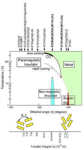
Figure 2 Lattice structure of the cation layer of θ-(BEDT-TTF)₂X. t_p and t_c are the nearest neighbor hopping integrals. (t_p, t_c)=(106, -5), (137, -49), and (99, -33) [meV] for CsCo, CsCo under pressure (10 kbar), and RbCo salts, respectively, according to the extended Hückel estimation [10]. V_p and V_c are the nearest-neighbor interactions, while V_a, V_q, and V_2c are the next-nearest-neighbor interactions. The a–c unit cell is the usual unit cell, while we can use the x–y unit cell to unfold the Brillouin zone.

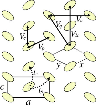
Figure 3 Horizontal stripe, vertical stripe, diagonal stripe, and c-axis threefold charge correlations. The green (or dark) molecules are the charge-rich ones.

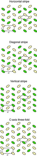
Figure 4 a-axis threefold (3×3 and 3×4) charge correlations. The dark molecules are the charge-rich ones.

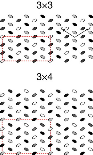
Figure 5 Upper panel: x-ray scattering intensity scanned along a diffuse sheet, expressed in units of the reciprocal lattice primitive vectors as with - 0.09ξ0.48, where the horizontal axis in the figure is h=-3+2ξ. q₁ is the wave vector corresponding to the a-axis threefold (3×3) correlation, while q₂ corresponds to the horizontal stripe correlation. Reproduced with permission from [10]. Copyright 1999 by the Physical Society of Japan. Lower panel: line (the arrow) along which the x-ray scan is taken (i.e. the diffuse sheet) shown in the Brillouin zone adopted in theoretical studies (see figure 7).

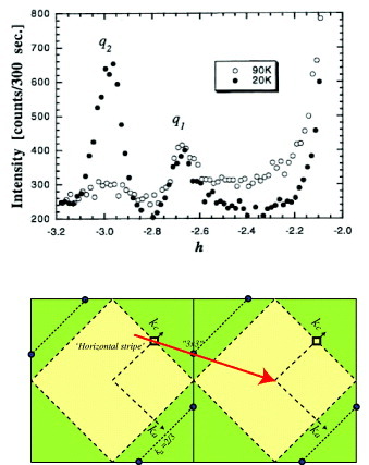
Figure 6 Effective lattice structure using the x–y unit cell. We specify the hoppings and the interactions by c, p, a, q, and 2c, which specify the positions relative to the center (red) site.

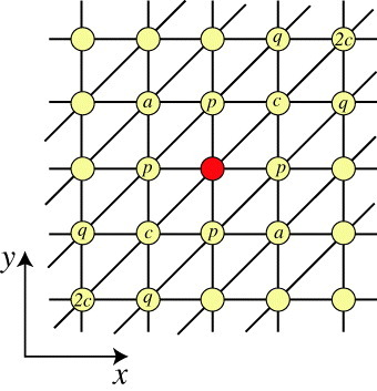
Figure 7 Upper panel: relation between the folded and unfolded Brillouin zone. Modulation wave vectors corresponding to various correlations are shown. The wave vectors are presented in units of the reciprocal lattice primitive vectors. The red line shows the Fermi surface for t_c=-0.3. Lower panel: Brillouin zone in the upper panel squeezed in the k_x=- k_y direction, and then placed repeatedly. The dashed lines represent the diffuse sheets observed at room temperature and below.

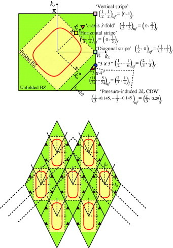
Figure 8 θ_d lattice. The hopping integrals are c1=1.5, c2=5.2, p1=16.9, p2=-6.5, p3=2.2, and p4=-12.3 in units of 10^-2 eV [11]. The green molecules are the charge rich ones in the horizontal stripe state.

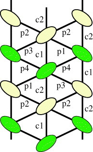
Figure 9 Ground-state phase diagram obtained by (a) variational Monte Carlo and (b) density matrix renormalization group for t_c=0, U=10, and V_a=V_q=V_2c=0. In (b), the diameter of the circles is proportional to the hole density at the hole-rich sites. (a) Reproduced with permission from [28]. Copyright 2006 by the Physical Society of Japan. (b) Reproduced with permission from [29]. Copyright 2008 by the American Physical Society.

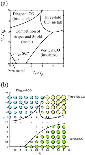
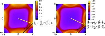
Figure 10 Contour plots of the RPA result of the charge susceptibility χ_c, the bare susceptibility χ₀, and the Fourier transform of the off-site interactions - V(q). t_c=- 0.3, U=3, V_p=1.3, V_c=1.5, V_a=V_q=V_2c=0, and T=0.05. The solid (dashed) arrow in χ_c(q) indicates the dominant (subdominant) peak at wave vectors close to (1/3, 1/3)_uf ((1/2, 0)_uf). The solid arrow in -V(q) is the wave vector (1/3, 1/3)_uf [30].

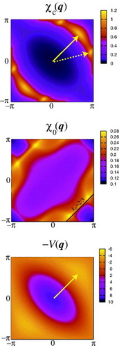
Figure 11 Contour plots of the RPA result for the charge susceptibility χ_c, the bare susceptibility χ₀, and the Fourier transform of the off-site interactions - V(q). t_c=- 0.3, U=4, V_p=1.8, V_c=2.0, V_a=0.4, V_q=0.7, V_2c=1.1, and T=0.25. The arrow in χ₀(q) indicates the peak position, i.e. the nesting vector of the Fermi surface. The arrows in -V(q) indicate the area at which -V(q) is broadly maximized [30].

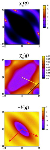
Figure 12 Plots similar to figure 11 except that t_c=-0.05 and T=0.15 [31].

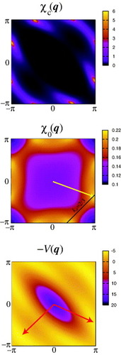
Figure 13 Comparison of the Fermi surface nesting between the cases of t_c=- 0.3 and -0.05.

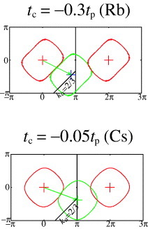
Figure 14 T_a-axis plotted as a function of t_c for U=4, V_p=1.8, V_c=2.0, V_a=0.4, V_q=0.7, and V_2c=1.1 [30]. t_p≃0.1 eV∼1000 K is taken as the unit of temperature. The values of t_c/t_p for X=MM′(SCN)₄ are taken from table II in [10]. For X=I₃, the value of t_p is taken from [5], while that of t_c is from ref. [38].

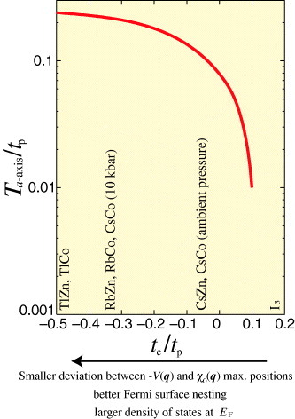
Figure 15 χ₀(q) for t_c=-0.05 at T=0.15 (∼150 K) (left) and at T=0.02 (∼20 K) (right).

MoriH 2006 J. Phys. Soc. Japan 75 051003 http://dx.doi.org/10.1143/JPSJ.75.051003

 Google Scholar

WatanabeMNogamiYOshimaKMoriHTanakaS 1999 J. Phys. Soc. Japan 68 2654 http://dx.doi.org/10.1143/JPSJ.68.2654

 Google Scholar

WatanabeMNodaYNogamiYMoriH 2004 J. Phys. Soc. Japan 73 116 http://dx.doi.org/10.1143/JPSJ.73.116

 Google Scholar

WatanabeHOgataM 2006 J. Phys. Soc. Japan 75 063702 http://dx.doi.org/10.1143/JPSJ.75.063702

 Google Scholar

NishimotoSShingaiMOhtaY 2008 Phys. Rev. B 78 035113 http://dx.doi.org/10.1103/PhysRevB.78.035113

 Web of Science ®Google Scholar

KurokiK 2006 J. Phys. Soc. Japan 75 114716 http://dx.doi.org/10.1143/JPSJ.75.114716

 Google Scholar

KobayashiATanakaYOgataMSuzumuraY 2004 J. Phys. Soc. Japan 73 1115 http://dx.doi.org/10.1143/JPSJ.73.1115

 Google Scholar

MoriHTanakaSMoriT 1998 Phys. Rev. B 57 12023 http://dx.doi.org/10.1103/PhysRevB.57.12023

 Web of Science ®Google Scholar

MoriH private communication.

 Google Scholar