Figures & data
Figure 1. To perform a microarray experiment, first, fragments of single stranded DNA are arranged in an array and bounded on a glass slide. They serve as probes. During gene expression a certain amount of mRNA occurs in the cytoplasm of target tissue cells. Reference mRNA is isolated from healthy cells of a tissue. Test mRNA is gained from the tissue related cancer cells. The mRNA from reference and test samples are converted into cDNA by reverse transcription, labelled with different fluorescent dyes and mixed together. Then the mixture is incubated with the single stranded DNA on the microarray slide. The different cDNA molecules hybridize competitively with the respective complementary DNA parts and the colours indicate different states of gene expression.
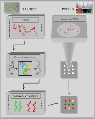
Figure 2. Left top: scan of a microarray. Green dye was used for the cDNA extracted from the reference cells and red dye was used for the cancer cells. Red spots indicate induced genes in cancer cells, green spots indicate repressed genes and yellow spots indicate no change between healthy cell and cancer cells. Right top: the microarray samples are converted into the expression matrix. In the expression matrix, the genes are arranged in the rows and the columns represent the gene expression values. Left bottom: the gene expression matrix can be clustered in two ways: if the genes are clustered, then the similar gene expression patterns are grouped together. By clustering according to the samples, all cells with similar gene expression profiles are grouped together. Right bottom: by clustering the unstructured gene expression matrix (left), the genes with similar expression patterns are grouped together in a structured data set (right).
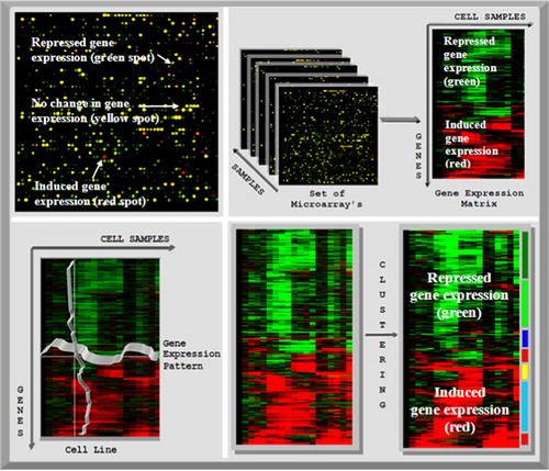
Figure 3. Left top: every gene is represented by a point in a P dimensional space, where the position of the point is determined by the P expression values xk on each axis of the coordinate system. Right top: a support vector machine tries to find a hyperplane which separates two predefined classes of genes in a training set. The first class is labelled positive and the second class is labelled negative. The genes (with double edges) in each class that are closest to the hyperplane are called support vectors. Bottom left and right: if genes cannot be linearly separated in the initial expression space, their vectors are mapped in a higher dimensional space spanned by all products, with a predefined factor, of the expression values. In this space a hyperplane separating the instances can be found.
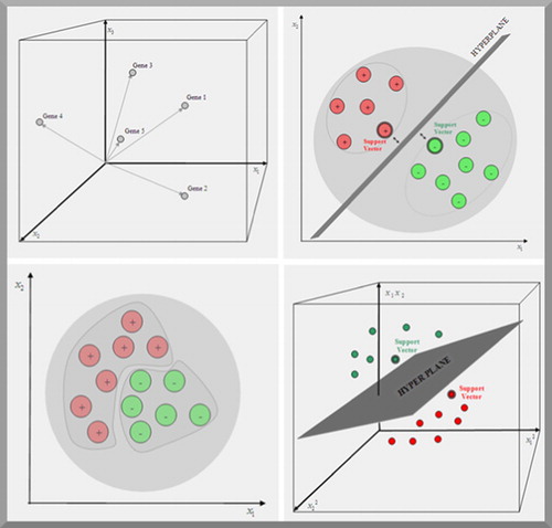
Figure 4. Kaplan–Meier plot of patients, treated for diffuse large B-cell lymphoma. The plot shows two distinct clinical outcomes. The patients respond differently to the chemotherapy and segregate into high clinical risk and low clinical risk categories depending on the number of years survival post-diagnosis. By separating the patients with microarray analysis into germinal centre B-like and activated B-like subcategories of diffuse large B-cell lymphoma, it is shown that the two clinical outcomes agree with the two subcategories.
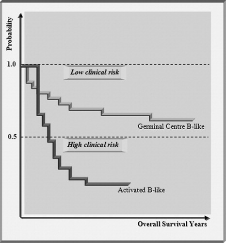
Figure 5. Signature genes are a set of genes with distinct expression patterns, which are used for describing particular cell types. Two signature genes, the germinal centre B cell and the activated B cell are identified and used for clustering the samples (containing normal and malignant lymphomas) into two subcategories. The subcategories are characterized by cell type and cell process. For this purpose, the genes are clustered first according to their expression patterns and additionally the samples are clustered according to the similarity of their gene expression profiles. The cluster analysis shows that the diffuse large B-cell lymphoma samples are completely contained in the germinal centre B-cell cluster (cell type).
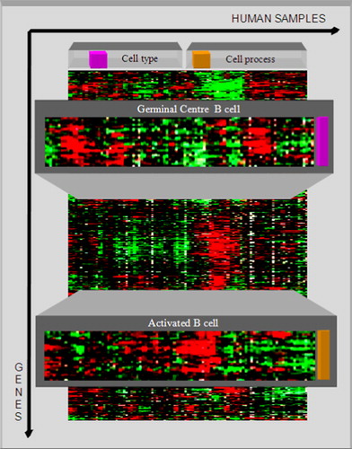
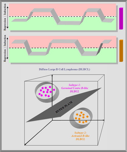
Figure 6. By use of the germinal centre B-cell signature gene, the diffuse large B-cell lymphoma (DLBCL) samples are clustered into two subcategories: germinal centre B-like DLBCL and activated B-like DLBCL. The different gene expression patterns are clearly shown.
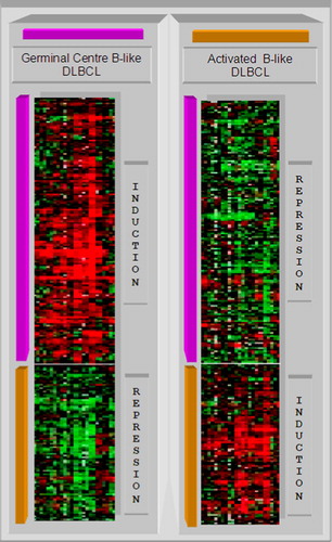
Figure 7. Top: the overall behaviour of the signature genes is shown in the plots. The germinal centre B-cell signature gene shows a repression of the expression in the first columns, an induction in the next columns, then a repression followed by an induction and a repression in the next columns. The activated B-cell signature gene shows a negative correlation with this pattern. Bottom: during the training phase, a support vector machine generates a maximum margin hyperplane that separates the germinal centre B cells and activated B cells diffuse large B-cell lymphomas (DLBCL).