Primary Succession Following Deglaciation at Koryto Glacier Valley, Kamchatka

Figures & data

FIGURE 1 (Top) Location of the Koryto Glacier in the Kronotsky Peninsula, eastern Kamchatka. (Bottom) Northwestward view of the Koryto Glacier Valley in mid-August 1999.

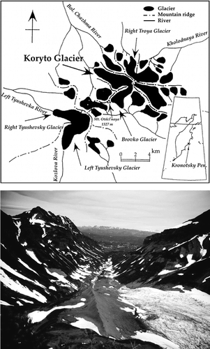
FIGURE 2 (Top) Close-up view of the deglaciated foreland with Alnus fruticosa stands. (Bottom) Detailed map of the deglaciated foreland with terminal and lateral moraines.

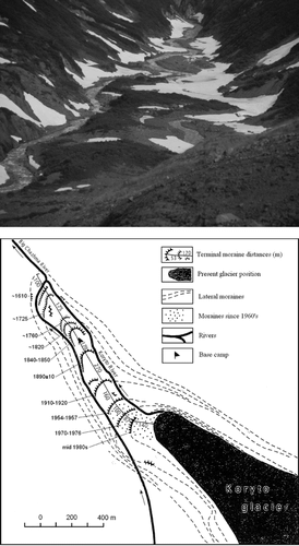
TABLE 1 Total carbon and nitrogen concentrations (mg g⁻¹) from soil horizons within moraines of the Koryto Glacier foreland. C—soil parent material just above bedrock, B—illuvial horizon, A—eluvial dark colored horizon, L-H—litter/humus horizon.

FIGURE 3 List of plant families participating during the succession with the number of species (white bar) and share of total vegetation cover (black bar). Also shown is the number of species for each family in the local species pool (gray bar).

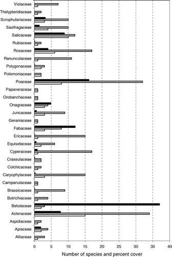
TABLE 2 Species frequency of occurrence (% of plots in each community for 32 major species from a total of 85) for the eight vegetation communities on the Koryto Glacier foreland.

TABLE 3 The eight vegetation communities derived from TWINSPAN and their characteristics: age of moraines on which they were located, mean (±SD) and maximum number of species per 2.5-m × 2.5-m plots, Shannon diversity and evenness, Simpson dominance, vegetation disimilarity (Chord distance), % proportion of seven growth forms, mean plant cover, and substrate and edaphic characteristics.

TABLE 4 Between-site comparison of Alnus fruticosa leaf traits (mean ± SE), ring counts (stem base, 70 and 140 cm), and mean ring width (min–max). Shown are also vegetation and soil characteristics for two types of stands A: Alnus coverage > 40%, and B: Alnus coverage < 40%. ns—non-significant differences among moraines (P > 0.05), ▴significant increase, ▾decrease, or • peak in the values of tested characteristics.

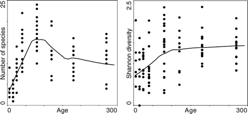
FIGURE 4 DCA–ordination diagrams: (a) pattern of compositional similarity between samples of successional vegetation (different symbols denote different Twinspan communities [1-○, 2-□, 3-◊, 4-l, 5-•, 6-▪, 7-♦, 8-□]; the first two ordination axes accounted for 12.9 and 9.7% of variability, respectively); (b) successional changes in species diversity; (c) plant species optimum performance; and (d) relationships to environmental factors and proportions of seven growth forms, with isoclines of species richness of samples.

TABLE 5 Canonical correspondence analyses of compositional variability in primary successional vegetation. Analyses were conducted for all plots (1–9) and for each moraine separately (10–16). Explained variability and significance levels (*** P < 0.001, ** P < 0.01, * P < 0.05) are shown for the marginal effects—variability explained by a given factor without considering other factors, and the partial (net) effects—variability explained by a given factor after accounting for the effects of other factors (covariables). In analyses 10–16, significant factors selected by forward selection are shown.

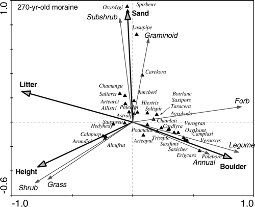
FIGURE 5 CCA ordination diagram displays the relationship between species cover and significant environmental factors on the 270-yr-old moraine. Growth form proportions were made passive so as not to influence the ordination axes, but their relation to dependent and explanatory variables can be judged from the ordination diagram. For abbreviation of species names see Table 2. The remaining species: Phlealpi—Phleum alpinum L., Allistric—Allium strictum Schard., Oxyrdygi—Oxyria dygina L., Spirbeau—Spirea beauverdiana Scheid., Taracera—Taraxacum ceratophorum (Ledeb.) DC., Botrlanc—Botrychium lanceolatum (Gmel.) Angstr., Luzupipe— Luzula piperi (Cov.) Jones., Agrokudo—Agrostis kudoi Honda, Camplasi—Campanula lasiocarpa Cham., Veraoxys—Veratrum oxysepalum Turcz., Polebore—Polemonium boreale Adams.

FIGURE 6 Changes in recorded number of species and calculated Shannon diversity indices with surface age of moraines. The curves were fitted by local polynomial regression fitting (loess).