The Physical Limnology and Sedimentology of Meziadin Lake, Northern British Columbia, Canada

Figures & data

FIGURE 1. Meziadin Lake (34 km², 244 m above sea level) and its drainage basin (530 km²). The largest inflow of water comes from the Strohn Creek drainage, including its tributary Surprise Creek (230 km², of which 50.5 km² [22%] is glacier covered [gray shading on map]). Inset map of British Columbia indicates the location of the lake

FIGURE 2. Bathymetry of Meziadin Lake based on 60.3 km of acoustic sub-bottom survey. Locations of profiles of water temperature, conductivity and optical turbidity, sediment-trap moorings, water temperature monitoring site, and Ekman grab samples are indicated

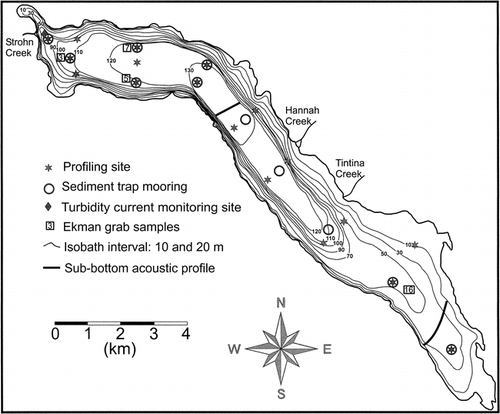
FIGURE 3. Discharge hydrograph for Strohn Creek and suspended sediment concentrations (SSCs) in Strohn and Surprise creeks at locations shown in Figure 1. Also shown is the mean daily air temperature at Smithers, 200 km south of Meziadin Lake

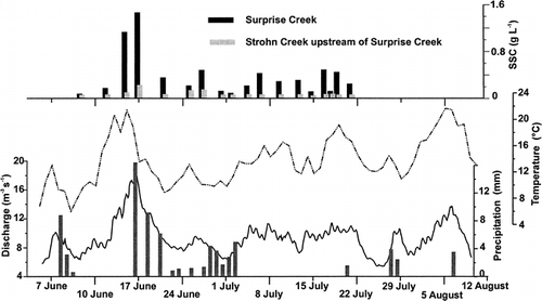
FIGURE 4. Transects along Meziadin Lake from the northwest (Strohn Creek inflow) to the southeast corner of the lake showing the suspended sediment concentration in mg L⁻¹ determined from optical transmissivity and the calibration obtained in nearby Bowser Lake (Gilbert et al., 1997). Inset on 17 June shows the cross-lake data at stations 5 and 7 (Fig. 2)

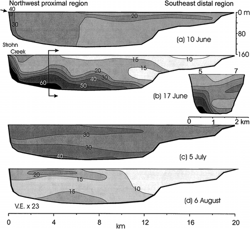
FIGURE 5. Discharge hydrograph for Strohn Creek and temperature 1 m above the lake floor at a site near the point of inflow (Fig. 2) illustrating the frequency of turbidity currents as peaks in temperature

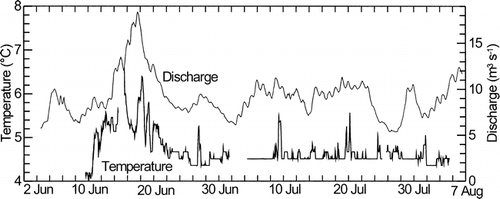
FIGURE 6. Mass accumulation rates (MARs) in Meziadin Lake from sediment traps located at 40-m depth and 1 m above the lake floor during the period 4 or 6 June to 8 August. Values of MAR (bold) represent the mean of 2 traps at each location. MAR in the upper traps is shown as a percentage of that in the lower traps at each site (parentheses). Accumulation during that period on the lake floor (italics) is derived from MAR based on a mean measured bulk density of 1210 km m⁻³ in 10 surficial samples of the lake floor. Trap numbers refer to discussion in text. Only the lower traps were deployed at site 11 due to the shallow water depth

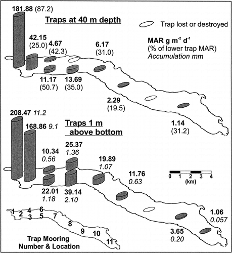
FIGURE 7. Particle size distributions (after Beierle et al., 2002) in sediment traps at sites 1 and 2 (Fig. 6). Values are in percent in 0.25 phi intervals; isopleth interval is 1%. Also shown is the geometric mean grain size (dots). Deposition began on 4 June and ended on 8 August when the traps were recovered. Reservoirs on 3 trap pairs were replaced on 3 July, providing a time marker as shown

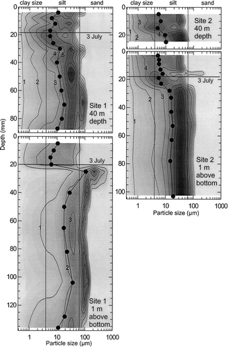
FIGURE 8. Particle size distributions (after Beierle et al., 2002) in four Ekman samples of surficial sediments from Meziadin Lake. Values are in percent in 0.25 phi intervals; isopleth interval is 1%. Also shown is the geometric mean grain size (dots). For locations see Figure 2

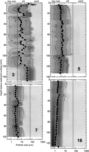
FIGURE 9. 3.5 kHz sub-bottom acoustic profiles (a) in the inflow-proximal region and (b) in the distal region of Meziadin Lake. Locations are shown on Figure 2. Depths in water and sediment assume a sound velocity of 1460 m s⁻¹. Numbers refer to acoustic facies described in the text. The dashed line marks the lowest reflecting surface interpreted as bedrock

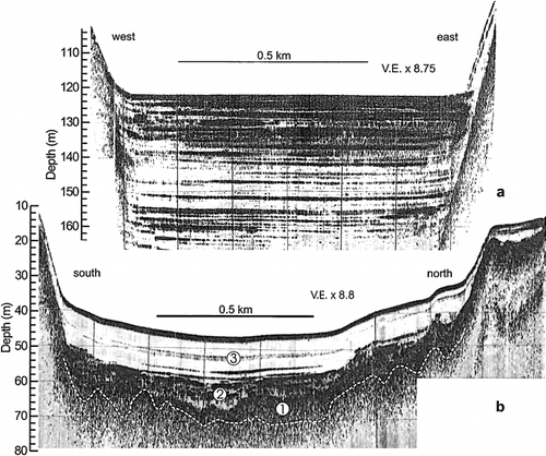
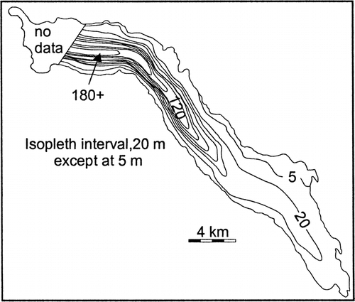
FIGURE 10. Total thickness of sediment in Meziadin Lake determined from sub-bottom acoustic survey

Gilbert, R. , J. R. Desloges , and J. J. Clague . 1997. The glacilacustrine sedimentary environment of Bowser Lake in the northern Coast Mountains of British Columbia, Canada. Journal of Paleolimnology 17:331–346.

 Web of Science ®Google Scholar

Beierle, B. D. , S. F. Lamoureux , J. M H. Cockburn , and I. Spooner . 2002. A new method for visualizing sediment particle size distributions. Journal of Paleolimnology 27:279–283.

 Web of Science ®Google Scholar