Figures & data
Figure 2 The figure illustrates the topography variability in the permafrost areas of southern Norway and the Alps. The topographic variation is expressed as the standard deviation of elevation within a 10 km radius from each point (cell in a DEM) in the map. The colored areas denote the areas potentially underlain by permafrost according to CitationBrown et al. (1995). While the mountains of southern Norway are dominated by an elevation standard deviation of below 300 m, the corresponding value for the Alps is above 300 m, with large areas above 500 m. The photographs display the difference of paleic and alpine landscapes, exemplified for southern Norway (Dovrefjell) and Switzerland (Engadin). The dotted line shows the position of the profile of .
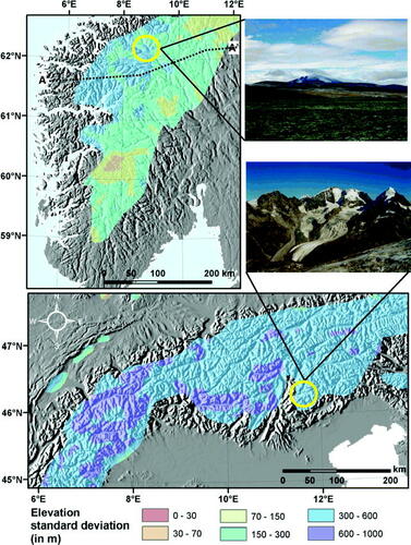
Figure 3 Example of the relation between equilibrium line altitude of glaciers (ELA) and lower limit of discontinuous mountain permafrost (MPA) along a west–eastern transect in southern Norway (based on CitationEtzelmüller et al., 2003, modified). The shaded areas denote locations of palsa mires as a morphological expression for sporadic permafrost. The numbers indicate: (1) the zone of dominating glacier coverage, (2) the zone of co-existing glaciers and permafrost, and (3) the zone of periglacial dominance and the absence of glaciers. Jb = Jostedalsbreen, SFj = Sognefjell, Jh = Jotunheimen, Ron = Rondane, Tf = Tronfjell, Fe = Femund area.
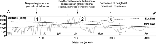
Figure 4 Conceptual diagram showing the relation between precipitation (continentality), temperature, glacier equilibrium line altitude (ELA), and permafrost (“cryosphere model,” modified based on CitationHaeberli and Burn, 2002). The shaded area denotes the zone where interactions between glacial processes and permafrost are to be expected. The dashed line marks the approximate transition between cold and warm firn. The dotted line crudely denotes the timberline. The circles indicate areas mentioned in this paper. NM = northern Mongolia, EY = eastern Yukon, WY = western Yukon, WN = western Norway, EN = eastern Norway, FM = Finnmark county in northern Norway, IS = northern and eastern Iceland, AL = Alps. The pictures illustrate the diversity of mountain permafrost settings throughout selected sites in the northern hemisphere.
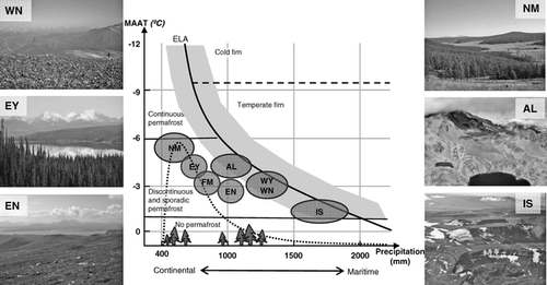
Table 1 Statistical relation between environmental factors and permafrost existence in different mountain settings. The relations are extracted from literature, and mainly based on linear or logistic regression analysis of permafrost proxies (bottom temperature of the snow cover [BTS], rock glaciers) and permafrost existence. ++/−− = strong positive or negative statistically significant relation, +/− = statistically significant relation, 0 = weak or no statistical significance.
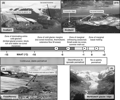
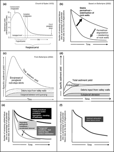
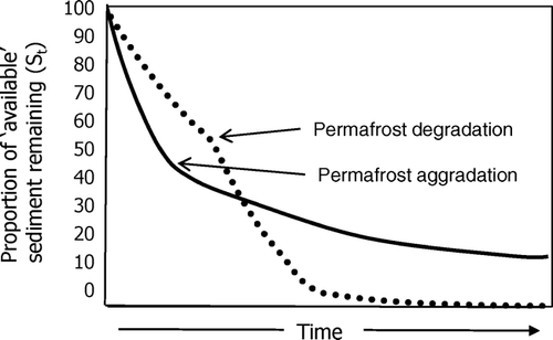
Figure 7 Theoretical and simulated exhaustion rates calculated with a time-dependant k(T) from Equation 2. In the “permafrost degradation” case, k changes linearly from 0.1 to 0.25 ka−1 between a certain time period. In the “permafrost aggradation” case, k changes linearly from 0.25 to 0.1 ka−1 .