Figures & data
FIGURE 1. Long-term monthly maximum and minimum air temperature means (± S.D.) and precipitation from 1955 to 1980 for the Barcroft weather station (3801 m elevation).
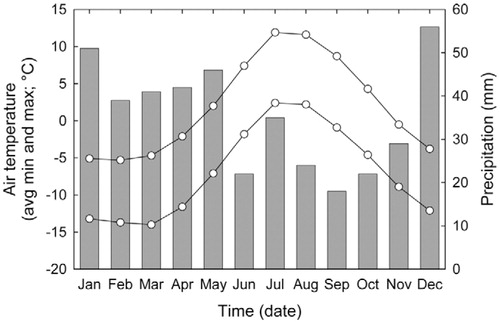
FIGURE 2. Alpine fellfield community on granite substrate at 3750 m elevation in the White Mountains, looking to the east across the Owens Valley to the snow-capped Sierra Nevada in the distance. (A) community surface characteristics; (B) cushions of Eriogonum ovalifolium; (C) mats of Penstemon heterodoxus; (D) upright leaves of Poa glauca; (E) small boulder with surrounding bare soil.
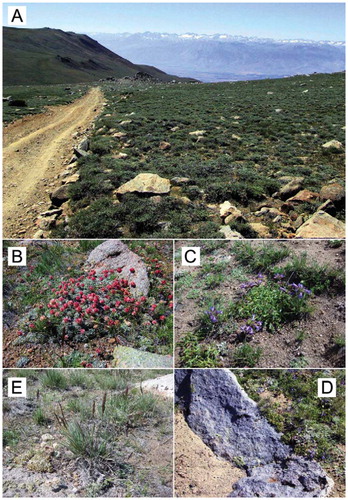
FIGURE 3. Cable-mounted mobile networked infomechanical systems (NIMS) rapidly deployable (RD) deployment with (A) support structures spanning the transect and (B) the infra-red sensor, showing support and guide cables and the festooned data cable.
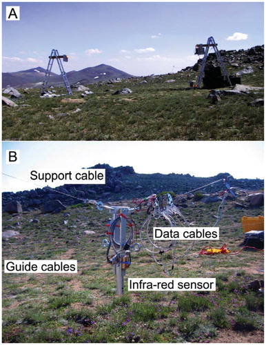
FIGURE 4. Hourly (A) air temperatures at 1 (solid black line), 10 (dashed black line), 30 (solid gray line), and 100 cm (dotted black line) above bare soil and (B) soil temperatures at the soil surface for a bare soil (solid black line), and at 10 cm depth in the soil below bare soil (dashed black line) and below Eriogonum ovalifolium (dotted black line) at the study site on 1–2 August 2005.
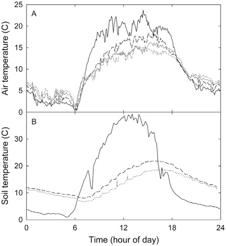
FIGURE 5. A 24-hour cycle of surface temperatures at a spatial resolution of 100 mm across a 3700 mm transect at the fellfield study site. Letters indicate locations where 100% cover of substrate or vegetation type was identified by digital images taken of the transect and include (B) boulder, (S) bare soil, (E) Eriogonum ovalifolium, (P) Penstemon heterodoxus, and (G) Poa glauca.
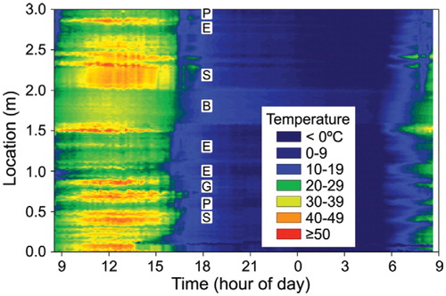
FIGURE 6. Hourly surface temperature across the entire transect. Depicted are the median (as the horizontal line between boxes), the 10th and 25th (as boxes) and the 75th and 25th (as error bars) percentile distributions, and all outliers (as points) of surface temperature. Data are from 308 locations along the transect with six time periods centered on the hour, approximately 10 min apart, averaged for each hour of measurement.
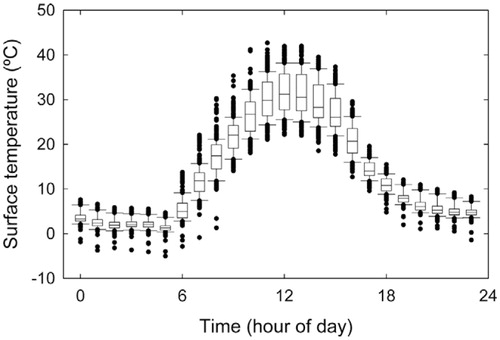
FIGURE 7. Frequency of temperature differences recorded between adjacent locations (A) 2 cm, (B) 5 cm, and (C) 10 cm distance apart along the transect during the time period when the maximum temperature was recorded (black bars; 12:05 h), and the time when the maximum standard deviation of temperature was recorded (gray bars; 13:52 h).
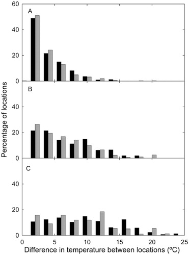
FIGURE 8. Mean temperature difference between air measured at 1 cm above bare soil and surface temperature at locations on the transect corresponding to (A) Penstemon heterodoxus, (B) Poa glauca, (C) Eriogonum ovalifolium, (D) boulder, and (E) bare soil. Data are means of 5 locations at the study site on 1–2 August 2005.
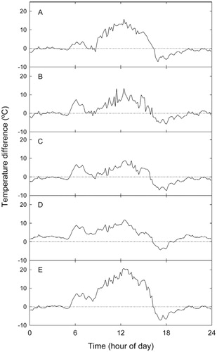
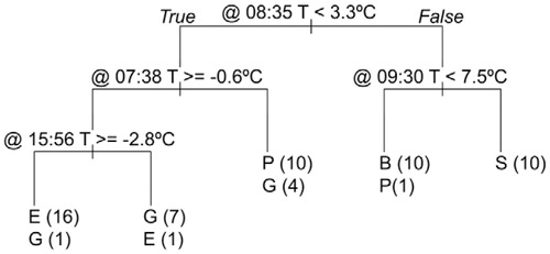
FIGURE 9. The classification results from the recursive partition decision tree analysis indicating the splits for separating the surface categories based on the difference between surface temperature and the air temperature at 1 cm height above bare soil (). Classifications are (B) boulder, (S) bare soil, (E) Eriogonum ovalifolium, (P) Penstemon heterodoxus, and (G) Poa glauca. Numbers in parentheses after each class indicate the number of instances of a location being classified into each category.