Lake Fluctuations, Plant Productivity, and Long-Term Variability in High-Elevation Tropical Andean Ecosystems

Figures & data

FIGURE 1. (A) Study area location in South America; (B) lakes (codes in capital letters, see Table 1), and dendrochronological sample sites used for the regional chronology (indicated with white dots); (C) geographical location of meteorological stations used for the analysis; and (D) Spearman correlation map between precipitation data from meteorological stations and the average of the differences of the six smaller lake sizes.

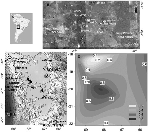
TABLE 1 Lakes measured in this study (with codes, see Fig. 1); minimum and maximum lake sizes; coefficient of determination (r ²); slope of size trend between 1985 and 2009; % of total lake size change in relation to initial value (2009–1985 size); and Pearson's correlation (r) with regional chronology ring width raw data.

TABLE 2 Pearson correlations between average of relative lake size for 1985–2009 period. For explanation of lake codes, see Table 1.

TABLE 3 Spearman correlation between interannual differences in average annual lake size and interannual variations in precipitation records (R) for 11 meteorological stations located along Bolivian and Chilean Altiplano (see Fig. 1, part D, for specific locations), regional precipitation average (R), and de Martonne's Aridity Index (AI performed for La Quiaca weather station). Countries codes: Bo—Bolivia, Ch—Chile, Ar—Argentina. For explanation of lake codes, see Table 1.

FIGURE 2. Trends in lake size, relative to maximum, for the 1985–2009 period. (A, B) Different groups of smaller lakes, (C) average of the six smaller lakes, and (D) larger lakes. Gray lines represent the linear regression.

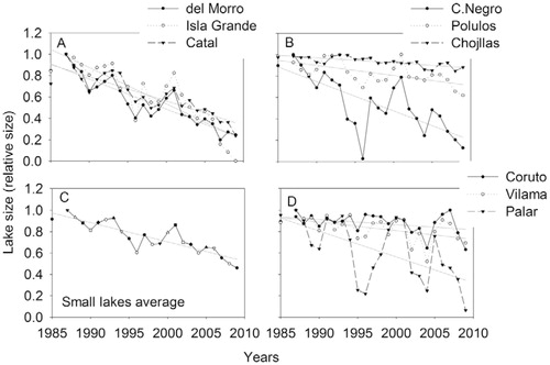
FIGURE 3. Relationship between lake size and meteorological data of the previous year. (A) Regional precipitation (averaged anomalies from the 11 meteorological stations with respect to the common period 1985–2009), (B) de Martonne's Aridity Index (based on La Quiaca station, 1985–2001 period) (size average of all lakes), and (C) mean temperature of La Quiaca (size average of the six smaller lakes).

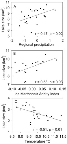
FIGURE 4. Temporal trends of TI MESAT parameters derived from the enhanced vegetation index (EVI) product from MODIS; (A) mean value (MV) and amplitude (AMP) (p < 0.05), and (B) total integral (TI) and growing season (GS) duration. Relationship between lake sizes (average of the six smaller lakes) and (C) MV and (D) AMP for the 2000–2009 period (p < 0.01).

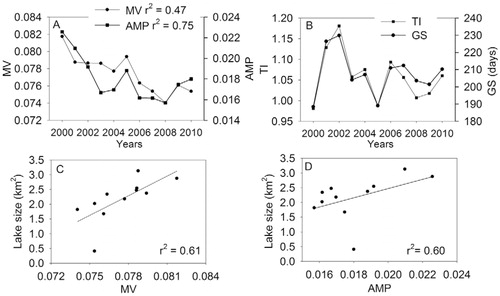
FIGURE 5. Relationship between P. tarapacana radial growth and indices of ecosystem function. (A) raw tree ring chronology vs. average lake size, (B) standardized tree ring chronology vs. differences in average of six smaller lakes sizes, and (C) raw tree ring chronology vs. EVI total integral.

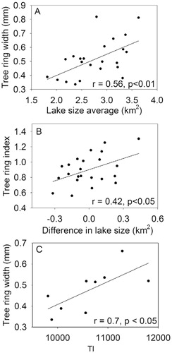
FIGURE 6. Regional chronology of Polylepis tarapacana (A) raw, and (B) standardized data, and (C) number of tree ring series (i.e. individual trees). Dark horizontal line indicates an adjusted curve of a 25-yr smoothing cubic spline to emphasize the low frequency variations. Vertical gray lines indicate years of growth reduction (one and two years after the occurrence of El Niño-Southern Oscillation [ENSO] events).