
Figures & data
FIGURE 1. Views of the Pyrenean study treeline in 1999 and 2009 showing standing dead trees and abundant tree regeneration.
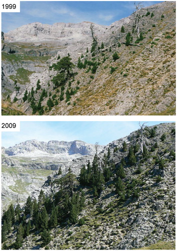
FIGURE 2. (a) Sampled Mountain pine stands in the Spanish Pyrenees (patches indicate the presence of Mountain pine) considering their distribution in two national parks (“Ordesa y Monte Perdido”, “Aigüestortes i Estany de Sant Maurici”) including the study site (Foratarruego, abbreviated as FR), and view of a dead Mountain pine (right inset). (b) Spatial pattern of Mountain pine recruits (circle size is proportional to age0.5) and standing dead trees with the corresponding point pattern analysis of saplings (observed pair-correlation function g(r) and 95% simulation envelopes obtained at different spatial scales). The latitude and longitude of study Mountain pine stands are shown in .
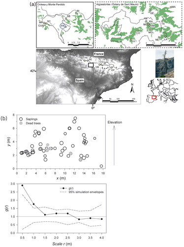
TABLE 1 Geographical, topographical, and ecological characteristics of the Mountain pine stands sampled across the Spanish Pyrenees (see sites in ). The study site (FR) is emphasized in bold characters. Values are means ± SD.
FIGURE 3. Probability of reproduction (cone presence) in treeline Mountain pine recruits as a function of their ages. According to the fitted binomial model (line, equation: y = e (52x-12.32)/(1 + e (0.52x-12.32), the probability of reproduction equal to 0.5 is reached at an age of 24 years as illustrated by the two arrows.
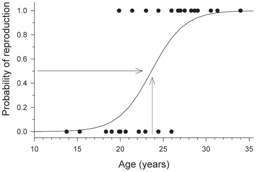
TABLE 2 Dendrochronological statistics obtained for the Mountain and Scots pine ring-width chronologies considering the common period 1900–2008.
FIGURE 4. Tree-ring width chronologies of Mountain and Scots pines displayed for their corresponding (a) well-replicated timespans and (b) temperature-growth relationships for both species. In the upper plot the residual indexed chronologies and their smoothed functions are shown (smoothing was done with 0.1-long loess functions). The right y-axis shows the number of sampled trees. The 20-year moving correlations calculated between both species chronologies are displayed with three probability levels shown as areas with different colors. In the lower plot, the bars show Pearson correlation coefficients calculated between monthly mean maximum (TMax) and minimum (Tmin) temperatures and ring-width indices from previous October up to current September during the period 1901–2008. Months abbreviated by lowercase and uppercase letters correspond to the prior and current years, respectively. The areas with different colors indicate significance levels.
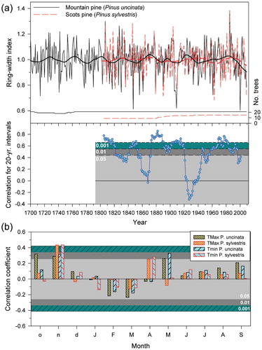
FIGURE 5. Trends of temperature anomalies in northern Spain and the Pyrenees derived from different proxies (red continuous line, speleothems; dendrochronologic reconstructions: black thin line, B-2008, CitationBüntgen et al., 2008; dashed thin line, DL-2012, CitationDorado Liñán et al., 2012) as compared with (a) the age structure of Mountain pines sampled in the Spanish Pyrenees (modified from CitationCamarero et al., 2015) and with (b) Mountain pine recruitment (births) and death events in the study treeline. In both panels age, recruitment, or death data are given in 20-year classes. The speleothem reconstruction was performed for northern Spain (CitationMartín-Chivelet et al., 2011). Dendrochronological reconstructions of maximum summer (June–August) temperatures (B-2008) and May–September mean temperatures (DL-2012) are based on maximum wood density and tree-ring width, respectively. The box in the x-axis of the lowermost plot indicates the period considered to analyze relationships between temperature and pine data.
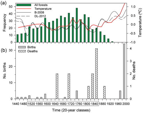
TABLE 3 Associations (Spearman correlation coefficients) observed between reconstructed temperature series, either based on dendrochronological (B-2008, CitationBüntgen et al., 2008; DL-2012, CitationDorado Liñán et al., 2012) or non-dendrochronological proxies (espeleothems, CitationMartín-Chivelet et al., 2011), and the age structure of Pyrenean mountain pine forests or the frequency of trees germinated (births) or dead (deaths) in the study treeline. The P value of each correlation is indicated between parentheses.