Soil Temperature and Soil Moisture Patterns in a Himalayan Alpine Treeline Ecotone

Figures & data

FIGURE 1. Study area and monitoring sites for soil temperature and soil moisture in Rolwaling Himal, Nepal. Experimental design includes two investigated altitudinal transects (NE = northeast exposition [black], NW = northwest exposition [red]) including four altitudinal zones (A, B, C, D), and location of experimental plots and climate stations (btm = bottom, top, Gompa, Na,Yalung). The map is adopted and modified from Müller et al. (2016).

FIGURE 2. Experimental design. Schematic illustration of the two different altitudinal transects (NE = northeast exposition, NW = northwest exposition) including four experimental plots (20 m × 20 m), respectively, in each altitudinal zone (A, B, C, D). Plot design (right) is equivalent on each plot. Koubachi Wi-Fi plant sensors are available on both transects.

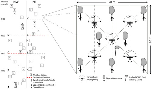
FIGURE 3. Daily mean soil temperatures during growing season in 2013, 2014, and 2015 at 10 cm depth in altitudinal zones A (closed forest), B (uppermost closed forest), C (krummholz), and D (alpine tundra) on NE (top) and NW transect (bottom). Treeline GSMT = growing season mean temperature at 10 cm soil depth at treeline.

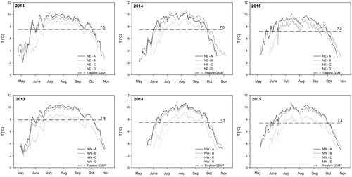
FIGURE 4. Spatiotemporal distribution of soil temperatures at 10 cm depth. A, B, C, D = altitudinal zones. NW = northwest. NE = northeast. MAM = spring (March, April, May), JJAS = summer (June, July, August, September), ON = autumn (October, November), DJF = winter (December, January, February).

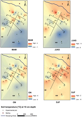
TABLE 1 Mean seasonal soil temperatures (± s.e.) at 10 cm depth in the altitudinal zones A, B, C, and D on the NE and NW transect. Different letters indicate significant differences at p < 0.05 by Post-hoc Nemenyi (Tukey) test.

TABLE 2 Mean (± s.e.) seasonal soil pF at 10 cm depth, and soil water content (SM) and available water capacity (AWC) in Vol.% or L m2 dm^-2 in the altitudinal zones A, B, C, and D on the NE and NW transect. AM 13 = April-May 2013, JJAS = summer (June, July, August, September), ON = autumn (October, November), DJF = winter (December, January, February), MAM = spring (March, April, May). Different letters indicate significant differences at p < 0.05 by Post-hoc Nemenyi (Tukey) test.

TABLE 3 Summary of vegetation, soil texture, and bulk density data (means of altitudinal zones + s.e.). Soil texture and bulk density were used for calculation of soil moisture (SM) and available water capacity (AWC) at 0–10 cm soil depth, dbh = diameter at breast height. NE = northeast, NW = northwest. A, B, C, D = altitudinal zones. Different letters indicate significant differences at p < 0.05 by Post-hoc Nemenyi (Tukey) test.

FIGURE 5. Spatiotemporal variation in available water capacity (Vol.% or L m^-2dm^-1). A, B, C, D = altitudinal zones. NW = northwest. NE = northeast. MAM = March–May, JJAS = June–September, ON = October–November, DJF = December–February.

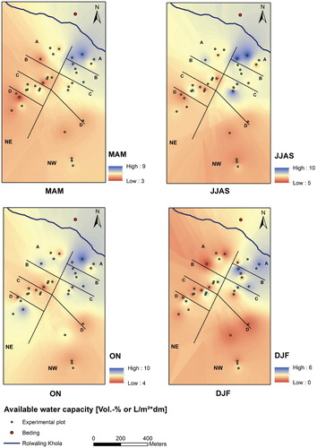
FIGURE 6. Results from redundancy analysis (RDA) with regard to (a) altitudinal zones, and (b) exposition. Blue arrows represent the independent explanatory variables soil temperature (ST), and available water capacity (AWC) gained as best explained principal components from preceding principal component analysis (PCA). The dependent response variables diameter in breast height (dbh), leaf area index (LAI), tree height, crown width, crown length, and number of tree individuals (Individuals) are colored in red. Circles combine related groups of sites (NE = northeast, NW = northwest. A, B, C, D = altitudinal zones). Scaling = 2 (in programming language R).

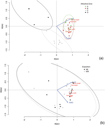
TABLE 4 Results of multivariate linear regression analyses, (a) The t and p values (T-test) are presented for relationships between explanatory variables (ST [soil temperature], AWC), and response variables. The explanation of the response variables is significant at a significance level of p = 0.05. (b) The best model for explanation of the response variables (ST, AWC, SM [soil moisture]) was produced by stepwise selection of independent variables. The results are highly significant at a significance level of p = 0.001 and p = 0.01, and significant at p = 0.05. LAI = leaf area index, dbh = diameter in breast height.

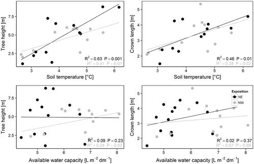
FIGURE 7. Scatter plot matrices showing simple linear regressions (R²,P-value) between soil temperature (ST) and available water capacity (AWC), respectively, and tree height and crown length, respectively, with regard to exposition. NE = northeast, NW = northwest, m = meter, L m^-2 dm^-1 = liter per square meter per decimeter.

Müller, M. , Schickhoff, U. , Scholten, T. , Drollinger, S. , Böhner, J. , and Chaudhary, R. P. , 2016: How do soil properties affect alpine treelines? General principles in a global perspective and novel findings from Rolwaling Himal, Nepal. Progress in Physical Geography , 40(1): 135–160.

 Web of Science ®Google Scholar