Quantitative Ultrasound Delta-Radiomics During Radiotherapy for Monitoring Treatment Responses in Head and Neck Malignancies

Figures & data

Table 1. Patient, disease and treatment characteristics for the study participants.

Patients and tumor characteristics n = 36 (all subjects)	n (%)
Age (years):   – Median (range)	60 (40–82)
Sex:   –Males   –Females	33 (92) 3 (8)
Site:   –Oropharynx   –Larynx   –Hypopharynx   –Left parotid   ––Nasopharynx   –Carcinoma unknown primary	26 (72) 4 (11) 2 (6) 1 (3) 1 (3) 2 (5)
Human papillomavirus:   –p16+   –p16-   –Not specified/–unclear	24 (67) 1 (3) 11 (30)
Stage
Primary tumor (T):   –T0   –T1   –T2   –T3   –T4	2 (5) 9 (25) 15 (42) 5 (14) 5 (14)
Node involvement (N):   –N1   –N2   –N3	21 (58) 10 (28) 5 (14)
Systemic therapy
Chemotherapy:   –Cisplatin (high and low dose)   –Carboplatin   –Carboplatin + etoposide   –Cisplatin + carboplatin	25 (69) 1 (3) 2 (5) 2 (5)
EGFR inhibitor:   –Cetuximab	1 (3)
None	5 (14)
Response at 3 months
Treatment response classification:   –CR   –PR	14 (39) 22 (61)

CR: Complete responders; EBV+: Epstein–Barr virus-positive carcinoma; N: Nodal staging (AJCC 8th edition); p16+: Human papillomavirus-positive tumor; PR: Partial responders; T: Primary tumor staging (American Joint Committee on Cancer [AJCC] 8th edition).

Figure 1. Kaplan–Meier survival plot showing recurrence-free survival for the complete responder and partial responder.

Figure 2. Quantitative ultrasound parametric maps.

Representative QUS parametric image overlays of ΔSI, ΔSAS and ΔASD at baseline, 24 h, week 1 and 4 of treatment for a complete responder (A) and a partial responder (B). The ultrasound B-mode images have been contoured to delineate the lymph node that was scanned.

ASD: Average scatterer diameter; QUS: Quantitative ultrasound; SAS: Spacing among scatterers; SI: Spectral intercept.

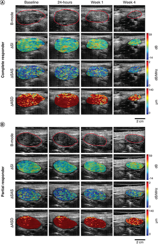
Table 2. Twenty four-hours post-treatment quantitative ultrasound mean spectral and texture values for the most significant features demarcating complete responders from partial responders.

Parameter	p-value	CR (mean ± SEM)	PR (mean ± SEM)
ΔSI-ENE	0.044	0.002 ± 0.001	-0.004 ± 0.030
ΔSAS-HOM	0.021	0.001 ± 0.002	-0.035 ± 0.030
ΔASD-COR	0.056	0.010 ± 0.008	-0.047 ± 0.038

Bolded parameters demonstrate statistical significance. Other features approach near significance.

ASD: Average scatterer diameter; CR: Complete responders; COR: Correlation; ENE: Energy; HOM: Homogeneity; PR: Partial responders; SAS: Spacing among scatterers; SEM: Standard error of the mean; SI: Spectral intercept.

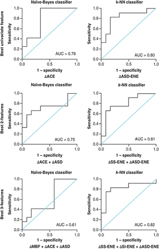
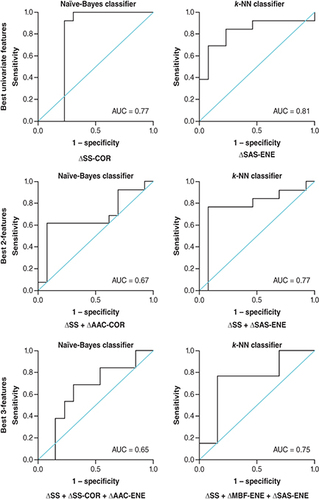
Table 3. Results for the best single-feature (A), two-feature (B) and three-feature (C) prediction models generated from machine-learning algorithms, K-nearest neighbor and naive-Bayes at 24-h post the first radiation treatment, week 1 and 4 of treatment.

A: single-feature classification
Classifier model	Time point	%Sn	%Sp	AUC	%Acc	Best univariate feature
naive-Bayes	24 h	77	83	0.67	80	ΔAAC-CON
	Week 1	85	86	0.77	86	ΔSS-COR
	Week 4	84	85	0.79	85	ΔACE
K-NN	24 h	75	70	0.74	72	ΔAAC-CON
	Week 1	75	85	0.81	81	ΔSAS-ENE
	Week 4	76	79	0.80	77	ΔASD-ENE
B: two-feature classification
Classifier model	Time point	%Sn	%Sp	AUC	%Acc	Best two features
naive-Bayes	24 h	67	73	0.64	70	ΔMBF + ΔAAC-CON
	Week 1	76	84	0.67	80	ΔSS + ΔAAC-COR
	Week 4	75	77	0.75	76	ΔACE + ΔASD
K-NN	24 h	74	78	0.78	76	ΔSS + ΔAAC-CON
	Week 1	73	78	0.77	76	ΔSS + ΔSAS-ENE
	Week 4	76	82	0.81	79	ΔSS-ENE + ΔASD-ENE
C: three-feature classification
Classifier model	Time point	%Sn	%Sp	AUC	%Acc	Best three features
naive-Bayes	24 h	63	69	0.63	66	ΔMBF + ΔSAS-CON + ΔAAC-CON
	Week 1	68	78	0.65	73	ΔSS + ΔSS-COR + ΔAAC-ENE
	Week 4	66	64	0.61	65	ΔMBF + ΔACE + ΔASD
K-NN	24 h	71	76	0.76	77	ΔSS + ΔSI-ENE + ΔAAC-CON
	Week 1	73	81	0.75	77	ΔSS + ΔMBF-ENE + ΔSAS-ENE
	Week 4	79	80	0.82	80	ΔSS-ENE + ΔSI-ENE + ΔASD-ENE

AAC: Average acoustic concentration; Acc: Accuracy; ACE: Attenuation coefficient estimate; ASD: Average scatterer diameter; AUC: Area under curve; CON: Contrast; COR: Correlation; ENE: Energy; HOM: Homogeneity; K-NN: K-nearest neighbor; MBF: Mid-band fit; SAS: Spacing among scatterers; SI: Spectral intercept; S_n: Sensitivity; S_p: Specificity; SS: Spectral slope.

Figure 3. Results for the best single-, two- and three-feature classification using naive-Bayes and K-nearest neighbor classifier models at 24 h after the initial radiation therapy treatment (receiver operating characteristic curve presented).

AUC: Area under the curve; CON: Contrast; ENE: Energy; K-NN: K-nearest neighbor; MBF: Mid-band fit; SAS: Spacing among scatterers; SI: Spectral intercept; SS: Spectral slope.

Figure 4. Results for the best single-, two- and three-feature classification using naive-Bayes and K-nearest neighbor classifier models at week 1 of radiation treatment (receiver operating characteristic curve presented).

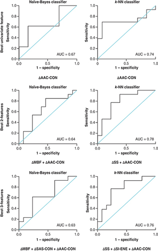
AUC: Area under the curve; CON: Contrast; COR: Correlation; ENE: Energy; K-NN: K-nearest neighbor; MBF: Mid-band fit; SAS: Spacing among scatterers.

Figure 5. Results for the best single-, two- and three-feature classification using naive-Bayes and K-nearest neighbor classifier models at week 4 of radiation treatment (receiver operating characteristic curve presented).

ACE: Attenuation coefficient estimate; ASD: Average scatterer diameter; AUC: Area under the curve; CON: Contrast; ENE: Energy; K-NN: K-nearest neighbor; MBF: Mid-band fit; SI: Spectral intercept.