Differences between the genomes of lymphoblastoid cell lines and blood-derived samples

Figures & data

Table 1 Pipeline software versions used

Pipeline versions	Assemblies per set
1.08.00.30	1
1.08.00.34	1
1.11.00.15	1
1.11.00.18	3
2.0.2.22	27
2.0.2.26	6
2.0.3.2	11
2.0.3.6	1
2.0.4.14	1
2.2.0.26	35
2.4.0.43	1
2.5.0.20	38

Table 2 Population distribution in the three sets of genome assemblies

Region	LCLs	MC1	MC2
EUR	125	117	112
AMR	1	8	12
EAS		1	1
SAS			1

Abbreviations: AMR, admixed American; EAS, East Asian; EUR, European; LCLs, lymphoblastoid cell lines; MC1 and MC2, matched control sets 1 and 2; SAS, South Asian.

Figure 1 Normalized coverage distributions.

Notes: LCLs display a wider distribution of average normalized coverages than matched controls (MC1 and MC2). Inset: standard deviations around the average coverage in the 90%–110% range.
Abbreviations: LCL, lymphoblastoid cell line; MC1 and MC2, matched control sets 1 and 2.

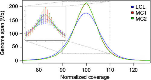
Figure 2 Software version effect.

Notes: Newer software versions have better ability to separate LCLs (blue) from matched controls (MC1 and MC2) by standard deviation of normalized coverage. Genome assemblies are arranged by assembly software version and chronologically.
Abbreviations: LCL, lymphoblastoid cell line; MC1 and MC2, matched control sets 1 and 2.

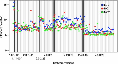
Figure 3 Chromosomal distribution of coverage deviations.

Notes: All autosomes except for chr19 display higher coverage variability (standard deviation of normalized coverage) in LCLs as compared to the control sets.
Abbreviations: LCLs, lymphoblastoid cell lines; MC1 and MC2, matched control sets 1 and 2.

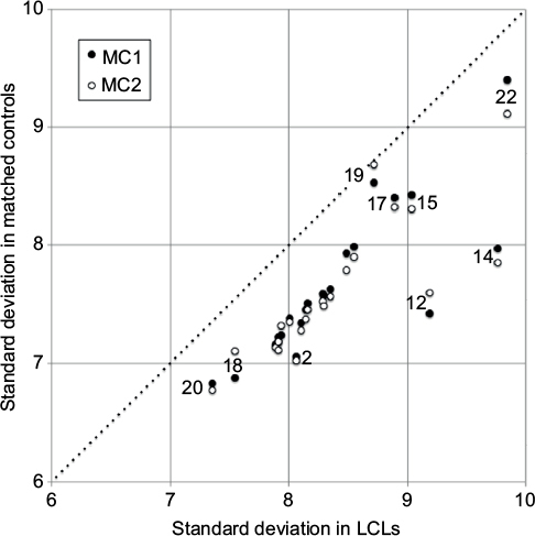
Figure 4 Genome set comparison along chromosomes.

Notes: (A) Smoothed KS statistic values (smoothing width=1000 bins=1 Mb) comparing LCLs to MC1 (blue), LCLs to MC2 (purple) and MC1 to MC2 (red) mapped along chromosomes 9 and 15; the inset chromosome ideograms show the increased KS values between LCLs and controls in early-replicating, light Giemsa bands. (B) Similar comparisons for chr6, highlighting regions of high dissimilarity between the normalized coverage distributions of LCLs and controls (lower left) and of similarity between all sets (lower right). Blue, red and green denote LCLs, MC1 and MC2, respectively.
Abbreviations: KS, Kolmogorov–Smirnov; LCLs, lymphoblastoid cell lines; MC, matched controls.

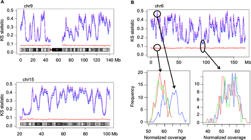
Figure 5 Correlation with various genomic parameters.

Notes: (A) Distribution of KS values grouped into 25 “GC buckets” (percentiles) of increasing GC percentage. (B) Distribution of KS values grouped by increasing distance to the nearest exon (square root scale). (C) Distribution of KS values grouped by replication timing ratio, log₂ (early/late). Lower values = late replication; higher values = early replication. (D) Distribution of KS values grouped by segmental duplication level, from 0 (outside segmental duplications, 94% of the genome) to 20 or more paralogous copies. The dashed line highlights the median KS value for the regions outside segmental duplications.
Abbreviations: KS, Kolmogorov–Smirnov.

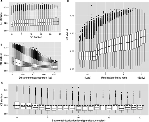
Figure 6 Example of regional coverage distortion.

Notes: Normalized coverage trace for one LCL (blue) vs its matched controls (red and green) in the 2p22.2 early-replicating band, averaged in overlapping 25 kb windows (upper panel). Blue points represent the actual 1 kb resolution normalized coverages for the LCL. Vertical lines connect to the transcription start sites of the known genes in this region (lower panel).
Abbreviations: LCLs, lymphoblastoid cell lines; MC, matched controls.

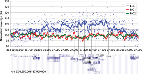
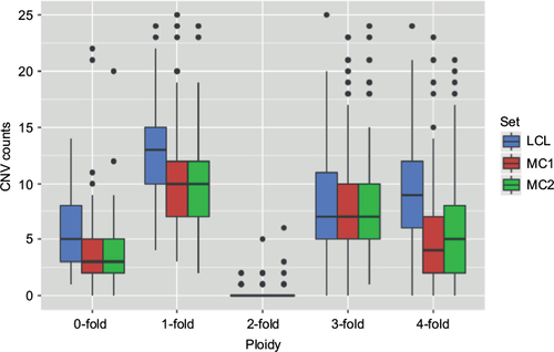
Figure 7 Effect on copy number calls.

Notes: Distribution of rare (frequency <1%) CNV counts in LCLs (blue) and controls (red and green), stratified by ploidy (0 to 4+ fold).
Abbreviations: CNV, copy number variant; LCLs, lymphoblastoid cell lines; MC, matched controls.