Current and emerging quantitative magnetic resonance imaging methods for assessing and predicting the response of breast cancer to neoadjuvant therapy

Figures & data

Figure 1 Lesion size measurement by MRI. (A) Unidimensional measurement of tumor long axis diameter. (B) Bidimensional measurement of tumor long and short axis diameters. (C) Three-dimensional measurement of tumor volume.

Abbreviation: MRI, magnetic resonance imaging.

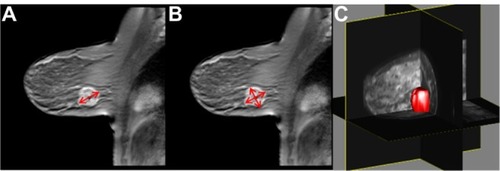
Figure 2 Fully quantitative DCE-MRI analysis in a breast cancer patient undergoing NAT. (A) Pretreatment DCE-MRI analysis yields a baseline calculated mean tumor K^trans value of 0.3 min⁻¹. (B) DCE-MRI analysis after one cycle of NAT yields a calculated mean tumor K^trans value of 0.2 min⁻¹. (C) Imaging after completion of NAT shows that the lesion is no longer visible; at surgery, the patient had a pathologic complete response.

Note: Ongoing studies are investigating whether early changes in mean tumor K^trans can reliably differentiate pathologic responders from nonresponders.
Abbreviations: DCE-MRI, dynamic contrast-enhanced magnetic resonance imaging; NAT, neoadjuvant therapy; K^trans, volume transfer constant.

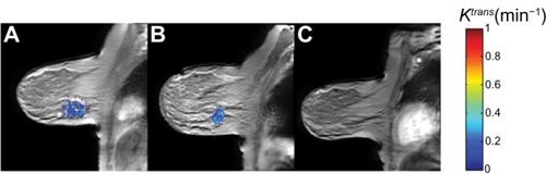
Figure 3 DW-MRI in a breast cancer patient undergoing NAT. (A) On a pretreatment image with no diffusion gradient (ie, b = 0 s/mm²), the tumor is difficult to distinguish from background normal parenchyma. (B) Pretreatment diffusion-weighted image (b = 660 s/mm²) demonstrates subtle patchy increased signal in the deep upper breast, corresponding to an infiltrative tumor. (C) Pretreatment quantitative ADC map, with color-coded voxels corresponding to tissue ADC. The tumor region is outlined in white. (D) ADC map derived from DW-MRI after one cycle of NAT; the tumor volume (again outlined in white) has markedly decreased.

Note: This patient went on to have a complete pathologic response.
Abbreviations: DW-MRI, diffusion-weighted magnetic resonance imaging; NAT, neoadjuvant therapy; ADC, apparent diffusion coefficient.

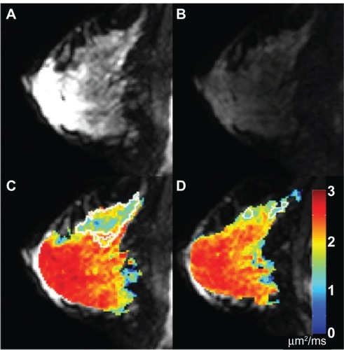
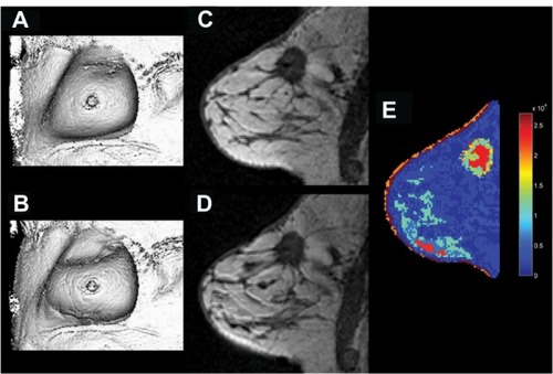
Figure 4 MT results from a healthy volunteer. (A) MT_off. (B) MT_on. (C) MTR map demonstrating an average 40% reduction in signal (ie, MTR = 0.4) in the fibroglandular tissue with good fat suppression.

Abbreviations: MT, magnetization transfer; MT_on, signal intensity with the saturation pulse; MT_off, signal intensity from the reference image; MTR, magnetization transfer ratio.

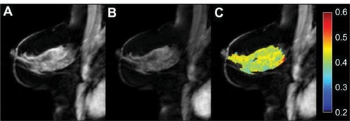
Figure 5 General pulse sequence diagram for a CEST MRI experiment.

Note: RF irradiation for a time t_s with an amplitude of B₁ precedes the excitation (α degrees) and image acquisition.
Abbreviations: CEST MRI, chemical exchange saturation transfer magnetic resonance imaging; RF, radiofrequency.

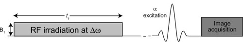
Figure 6 Example z-spectra arising from a CEST MRI experiment at 3 T.

Note: The normalized signal (S/S₀) is shown as a function of saturation offset frequency for regions of interest in malignant tumor (black line) and healthy fibroglandular tissue (gray line).
Abbreviations: CEST MRI, chemical exchange saturation transfer magnetic resonance imaging; S, signal intensity with saturation; S₀, signal intensity in the absence of saturation.

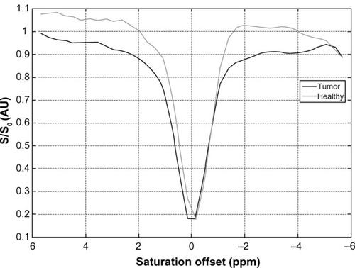
Figure 7 Amide proton transfer (APT) maps derived from CEST MRI in breast cancer patients undergoing NAT. Baseline (pretreatment) images are presented on the left, and images after one cycle of NAT are presented on the right. (A): patient with complete response after one cycle of therapy (27% decrease in measured APT from baseline). (B): patient with partial response (49% increase in measured APT). (C): patient with progressive disease (78% increase in measured APT).

Abbreviations: CEST MRI, chemical exchange saturation transfer magnetic resonance imaging; NAT, neoadjuvant therapy.

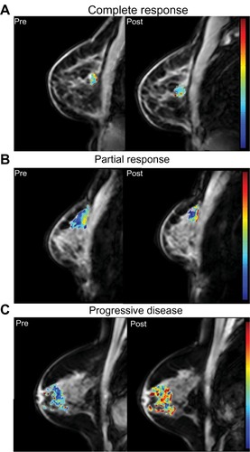
Figure 8 Static MRE (MIE) results from a breast cancer patient. (A) undeformed image volume. (B) deformed image volume. (C) undeformed central slice. (D) deformed central slice. (E) reconstructed tissue elasticity map.

Abbreviations: MRE, magnetic resonance elastography; MIE, modality-independent elastography.