Figures & data
Figure 1 Lip fullness was manipulated using the Face Liquify tool of Adobe Photoshop and ranged from (A) thinnest possible lips variant (minus 100) to (B) fullest possible lips variant (plus 100).
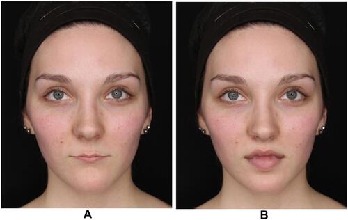
Figure 2 Comparison of presented levels of lip fullness offered by the graphics software (x-axis: from −100 to +100) with the participants’ assessments of lip fullness at the end of the experiment (y-axis: from 1 to 7). Pearson R coefficient for both experimental conditions indicate close to perfect fits. Confidence intervals (CI-95%) are additionally given by shadowed confidence bands (note: the band can hardly be perceived as it is in fact very narrow due to the near-to-perfect fit).
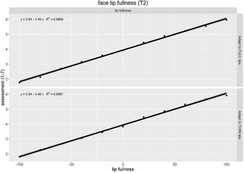
Figure 3 Mean data for face attractiveness (left) and face naturalness (right) for both adaptation conditions (top: Adapt_FullLips, bottom: Adapt_ThinLips), split by test phases (black: T1, red: T2). Data is modelled by second-degree polynomial functions—determination coefficient expressed as squared Pearson’s R is given for each curve fitting. Confidence intervals (CI-95%) are additionally given by shadowed confidence bands.
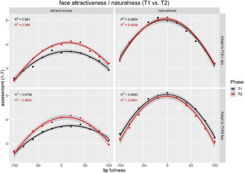
Table 1 Optimal Lip Fullness That Corresponds to the Mean (M) Maximum Values of the Employed Second-Order Polynomial Models for Each Participant, Adaptation Condition and Test Phase, Calculated for Both Dependent Variables (Attractiveness and Naturalness), Separately
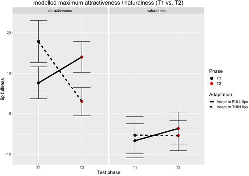
Figure 4 Mean values of individual optimal lip fullness for reaching a maximum for the respective dependent variables attractiveness (left) and naturalness (right). Solid lines show adaptation condition Adapt_FullLips and dashed lines the respective data for Adapt_ThinLips. Error bars indicate ±1 standard error of the mean.