Figures & data
Table 1 Five Steps Required for Random Hot Deck Imputation with Appropriate Confidence Interval Coverage
Table 2 Summary of Random Hot Deck Approach for Frequency, Sport, and Sport Count Variables. The Steps from Preliminary Donor Pool to Final Donor Pool and Applying the Sampling Method to the Data to Obtain the Imputed Value are the Same for Any Context or Study and are Omitted for Clarity
Figure 1 Imputation of activity frequency. (A) There is one week where frequency is missing (black row). Pain is coded as no pain in any location (No pain), new pain in at least one location (New pain), and old pain in at least one location but no new pain (Old pain). The individual had no pain in the week with missing data. The median frequency for the individual’s class and gender is calculated for the missing and surrounding weeks (Median Class Frequency). For the weeks with observed data, we also calculate the difference between the individual’s frequency and the median frequency (Freq minus Median Class Freq) as a measure of how much activity the individual does relative to their class and gender. (B) We match on nearby weeks with the same level of pain (gray rows). The preliminary donor pool is comprised of eight weeks where the individual also experienced no pain. (C) For simplicity of presentation, we chose a final donor pool that happened to exactly match the preliminary donor pool in (B). One of the weeks in the final donor pool is randomly selected (outlined in black). The difference between the individual’s frequency and the median class frequency for the sampled week is 1. This difference is imputed for the missing week. (D) The imputed frequency for the missing week is the sum of the median class frequency for the missing week and the imputed difference between the individual and median class frequency. In this example, the imputed difference of 1 is added to the median class frequency of 2 to obtain an imputed frequency of 3.
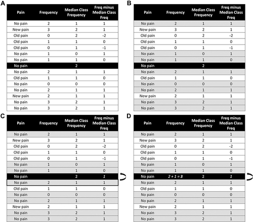
Figure 2 Imputation of sport. (A) There is one week where the sports performed are missing (black row). The individual had a total activity frequency of 2 in this week. (B) We match on closest frequency in the nearby weeks. The preliminary donor pool is comprised of weeks where the individual also had frequencies of 2 (gray rows). (C) For simplicity of presentation, we chose a final donor pool that happened to exactly match the preliminary donor pool in (B). One of these weeks is randomly sampled with equal probability (outlined in black). (D) The sports from the sampled week are imputed for the missing week.
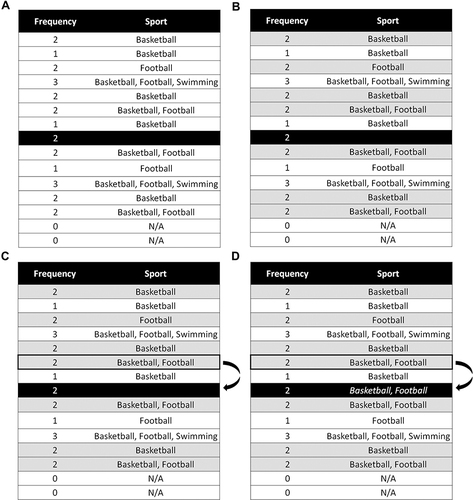
Figure 3 Imputation of sport where the number of sports is greater than the frequency. (A) There is one week where the sports performed are missing (black row). The individual had a total activity frequency of 2 in this week. (B) The preliminary donor pool is comprised of nearby weeks with the closest frequency to the missing week. Since there are no weeks with a frequency of 2, we match on weeks with frequencies of 3 (gray rows). For simplicity of presentation, we chose a final donor pool that happened to exactly match the preliminary donor pool in (B). One of the matched weeks is randomly sampled. (C) The sampled week has 3 sports, while the missing week only has a frequency of 2. The number of times in nearby weeks that the individual participated in each sport is determined. For weeks where the frequency is greater than the number of sports, the frequency is divided equally. The relative amount that the individual participated in each sport in nearby weeks is used as the sampling probability. Since the individual did basketball 10.5 times, football 7.5 times, and swimming 1 time, the probabilities are 55% (10.5/19), 40% (7.5/19), and 5% (1/19) respectively. (D) Sports are randomly sampled using the sampling probabilities and imputed for the missing week. Basketball and football are randomly imputed.
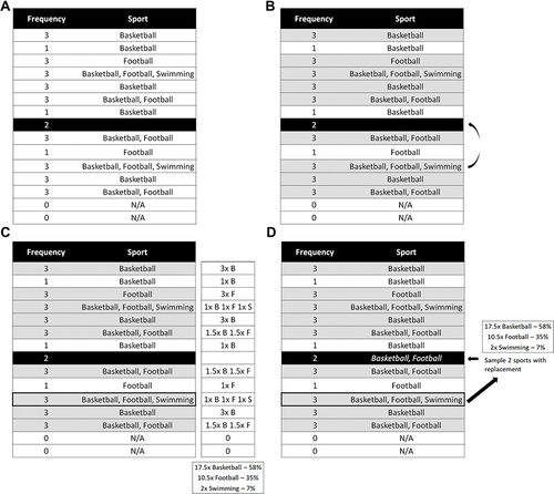
Figure 4 Agreement between gold standard and imputed datasets for sport by missingness pattern. “Overall” is a weighted average of the two missingness patterns (frequency data available, frequency data missing). Agreement was assessed between the gold standard and imputed datasets using an unweighted kappa. Points represent the average kappa across 5 imputed datasets, while bars represent the range of kappas between the 5 imputed datasets. The horizontal dashed line represents the cut-off for minimal agreement (kappa = 0.40) (McHugh 2012, Biochem. Medica.). Calculations were restricted to missing entries in the synthetic dataset; kappas calculated using the entire dataset ranged from 0.98 to 1.00. The percentage of entries where each sport was done in the gold standard dataset is shown below the plot.
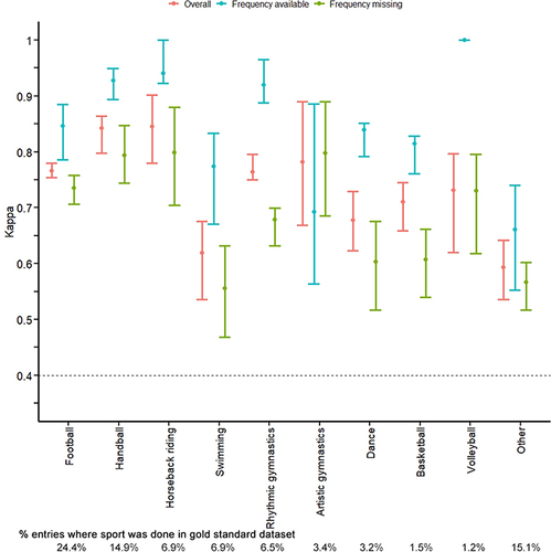
Figure 5 Imputation of sport counts where a single week is missing. (A) There is one week where the total frequency is greater than the number of sports performed (black row). We would like to impute individual counts for each sport that was done. (B) The individual participated in at least one session of basketball and one session of football. As the total frequency for the missing week is 3, we still need to impute a single count that is either basketball or football. (C) For simplicity of presentation, we chose a final donor pool that happened to exactly match the preliminary donor pool in (B). The relative proportion of each sport done in the missing week (basketball and football in (C)) is calculated for the nearby weeks and used as the sampling probabilities. As basketball was done 9 times and football was done 5 times, the probabilities are 64% (9/14) and 36% (5/14) respectively. (D) Basketball is randomly sampled for the missing sport. Sport counts are imputed as two sessions of basketball and one session of football.
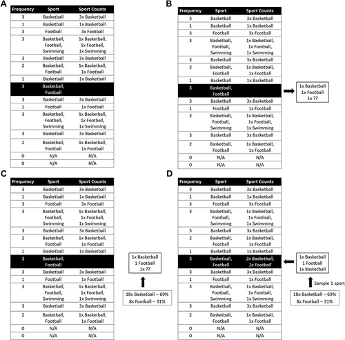
Figure 6 Imputation of sport counts where multiple weeks are missing. (A) There are two weeks where the total frequency is greater than the number of sports (black rows). We would like to impute individual counts for each sport that was done for both weeks. We focus on imputing sport counts for the first missing week. (B) In the missing week, the individual had a frequency of 3 and participated in basketball and football. They must have participated in one session each of basketball and football. We must therefore impute a single count. Sport counts are calculated for the nearby weeks. When the frequency is greater than the number of sports (ie for the week with frequency 4), the counts are evenly distributed (assigning 2 counts to basketball and 2 counts to football). (C) For simplicity of presentation, we chose a final donor pool that happened to exactly match the preliminary donor pool in (B). The relative proportion of each sport in the final donor pool (ie matching the sports that were done in the missing week) is calculated for the nearby weeks and used as the sampling probabilities. Since basketball was done 10 times and football 7 times, the sampling probabilities are 59% (10/17) and 41% (7/17) respectively. (D) Basketball is randomly sampled. Sport counts are imputed as 2 sessions of basketball and 1 session of football.
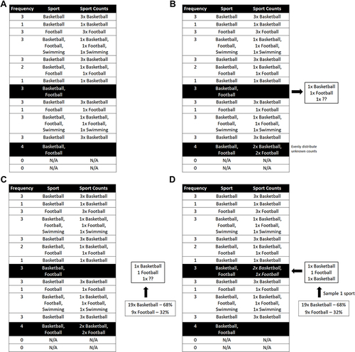
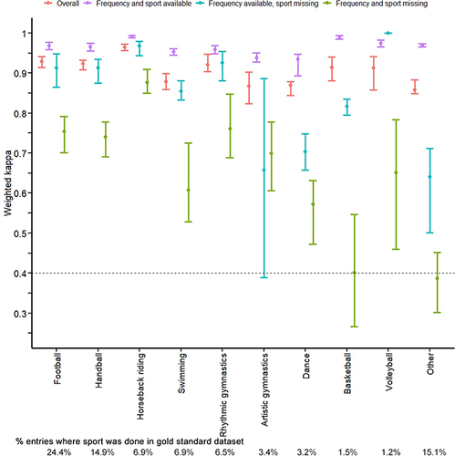
Figure 7 Agreement between gold standard and imputed datasets for sport count by missingness pattern. “Overall” is a weighted average of the three missingness patterns (frequency and sport data available; frequency data available but sport data missing; frequency and sport data missing). Agreement was assessed between the gold standard and imputed datasets using a weighted kappa. Points represent the average kappa across 5 imputed datasets, while bars represent the range of kappas between the 5 imputed datasets. The horizontal dashed line represents the cut-off for minimal agreement (kappa = 0.40) (McHugh 2012, Biochem. Medica.). Calculations were restricted to missing entries in the synthetic dataset; kappas calculated using the entire dataset ranged from 0.98 to 1.00. The mean sport count for each sport in the gold standard dataset is shown below the plot.