Figures & data
Figure 1 Schematic diagram of mouse acupoints. LI4, BL13, BL20, BL23, ST36, SP6 and LR3 are symmetrical on both sides of the body. LI4 is located between the first metacarpal bone and the second metacarpal bone of the forelimb; BL13 is located in bilateral intercostal region, directly below the third thoracic vertebra; BL20 is located in bilateral intercostal region, directly below the 11th thoracic vertebra; BL23 is located in bilateral intercostal area, directly below the second lumbar spine; ST36 is located at the posterolateral side of the knee joint, about 3mm below the head of the fibula; SP6 is located about 5mm above the straight point of the inner ankle of the hind limb. LR3 is located between the first and second metacarpal bones of the hind limb. Created using Biorender.com.
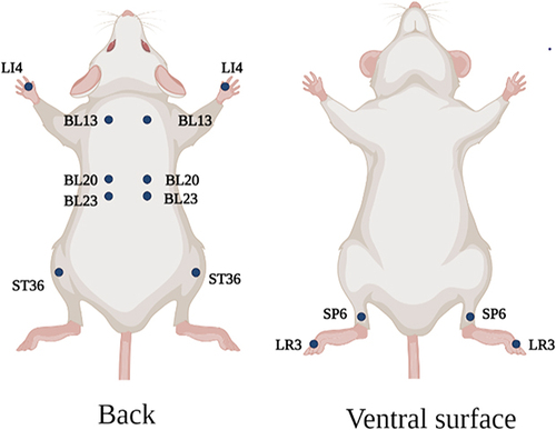
Figure 2 Effect of electroacupuncture on body weight and blood sugar of db/db mice. (a) Body weight changes before and after treatment. (b) Fasting blood glucose changes before and after treatment (c) Blood glucose values at each time point of OGTT; (d) AUC is calculated according to OGTT curve. (e) Serum insulin level was measured after treatment; (f) Calculate HOMA-IR index: HOMA-IR=FINS × FBG / 22.5; Data are expressed in mean ± standard deviation, #P < 0.05, ##P < 0.01 (n=8).
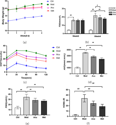
Figure 3 Effect of electroacupuncture on blood lipid in db/db mice. (a) Total cholesterol level (TC). (b) Triglyceride level (TG). (c) Low density lipoprotein level (LDL-C). (d) High density lipoprotein level (HDL-C). Data are expressed in mean ± standard deviation, #P < 0.05, ##P < 0.01 (n=8).
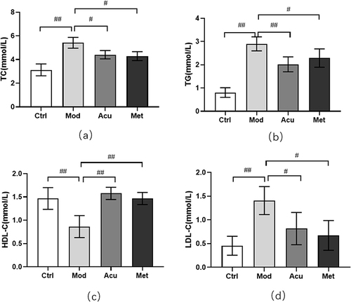
Figure 4 Analysis of microbial diversity of mice in each group. (a) The Venn diagram shows the number of 4 groups of OUT. (b) The Rank ambiguity curve shows the species distribution. (c) Alpha diversity analysis Observed specifications index. (d) Alpha diversity analysis Shannon index. (e) Beta diversity analysis NMDS diagram# P<0.05, ##P< 0.01 (n=5).
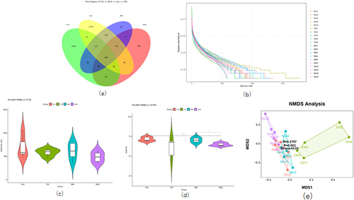
Figure 5 Structure and difference analysis of phyla horizontal flora. (a) Histogram of relative abundance of mouse flora composition at phyla level in each group. (b) Comparison of the relative abundance of Bacteroidetes. (c) Comparison of relative abundance of Firmicutes. (d) Relative abundance ratio of Firmicutes/Bacteroidetes. (e) Comparison of relative abundance of Epsilonbacteraeota. (f) Comparison of relative abundance of Actinobacteria. (g) Comparison of relative abundance of Tenericutes. (h) Comparison of relative abundance of Bacteroidota. # P<0.05, ##P< 0.01 (n=5).
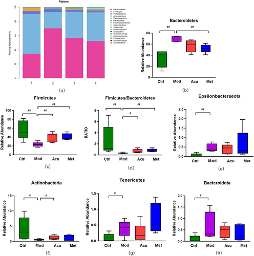
Figure 6 Structure and difference analysis of phyla horizontal flora. (a) Histogram of relative abundance of mouse flora composition at phyla level in each group. (b) Comparison of the relative abundance of Prevotellaceae_UCG-001 (c) Comparison of relative abundance of Alloprevotella. (d) Relative abundance ratio of Prevotellaceae_NK3B31_group. (e) Comparison of relative abundance of Bacteroides. (f) Comparison of relative abundance of Enterorhabdus. (g) Comparison of relative abundance of Clostridiales_vadinBB60_group_unclassified. (h) Comparison of relative abundance of Clostridiales_unclassified. (i) Comparison of relative abundance of Bilophila. (j) Comparison of relative abundance of Firmicutes_unclassified. (k) Comparison of relative abundance of Lachnospiraceae_unclassified. # P<0.05, ##P< 0.01 (n=5).
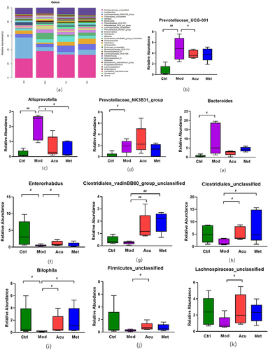
Figure 7 (a) Phylum and genus level mulberry map (b) Evolution branch tree generated by LEfSe.
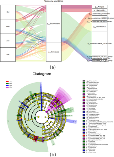
Figure 8 Analysis of fecal bile acid spectrum in each group of mice (a) PCA diagram of fecal bile acid composition in each group of mice (b) Content ratio of primary and secondary bile acids in mouse feces (c) Changes in fecal primary bile acid spectrum in each group of mice (d) Changes in fecal secondary bile acid spectrum in each group of mice (e) Changes in fecal secondary bile acid spectrum in each group of mice. # P<0.05, ##P< 0.01 (n=6).
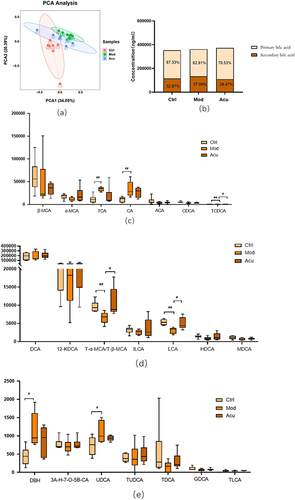
Figure 9 Correlation analysis between fecal bile acids and differential gut microbiota Spearman correlation values were used for the matrix. Significant correlations were noted by *p < 0.05, and **p < 0.01.
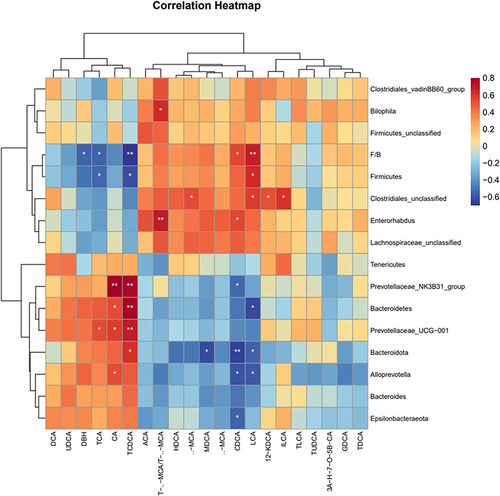
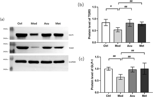
Figure 10 Expression of TGR5 and GLP1 proteins in each group of mice. (a) Representative Western blot brands of TGR5 and GLP-1 in the small intestine of db/db mice (b) The density analysis results of TGR5 in the small intestine of db/db mice (c) The density analysis results of GLP-1 in the small intestine of db/db mice. #P<0.05, ##P< 0.01.