Mutual information of local field potentials distinguishes area-V2 stripe compartments

Figures & data

Figure 1 (A–J) Relationships among single-unit tuning, local field potential (LFP) voltage, and LFP power.

Notes: (A) Tuning curves based on single-unit responses (mean firing-rate background) to luminance-contrast grating (2.0 cycles/degree) moved in both directions along six orientations. This cell (unit 1 at electrode 28) exhibited a peak response to the 0° grating. (B) Broadband LFP voltage as a function of time relative to stimulus onset in response to luminance gratings moved at six different orientations (S0 =0°, S5 =150°). Robust time-locked responses were observed in response to all stimuli. (C–F) Frequency band-limited LFP voltage as a function of time relative to stimulus onset for the six oriented grating stimuli. LFP responses were observed in response to all stimuli in each frequency band. However, the peak response, calculated relative to LFP voltage prior to stimulus onset, varied with the frequency band. (G–J) Frequency band-limited LFP power as a function of time relative to stimulus onset in response to the six oriented gratings. The latency, magnitude, and structure of the LFP-power responses varied across frequency bands.

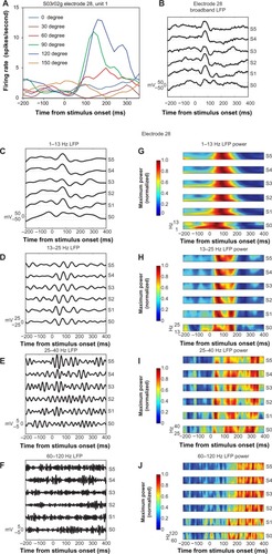
Figure 2 (A–C) Microelectrode-array electrode positions relative to cytochrome oxidase stripes.

Notes: (A) V2 stripes were identified from tangentially sectioned tissue stained for cytochrome oxidase (CO). Recording-site positions were then determined from the clear pattern of perforations made in the tissue by the array. (B) Optical density plot from the region of interest, indicated by the white rectangle in (A) that indicates the positions of the CO/optically dense thin and thick stripes, as well as the CO pale/optically brighter interstripes. (C) Location of CO-dense thin stripe superimposed on microelectrode-array electrode numbers. Based on their positions medial or lateral to the central thin stripe, the two CO-pale interstripes were distinguished as type II and type I interstripes, respectively.

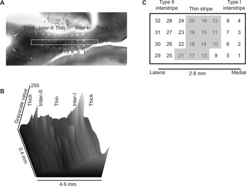
Figure 3 Linear component of mutual information encoded by local field potential (LFP) power in four frequency bands.

Notes: The linear component of mutual information varied systematically by electrode position and LFP frequency band. The linear information per electrode and frequency band is illustrated in the upper panel for the luminance-contrast stimulus set (stimuli 1–24), in the middle panel for the chromatic contrast stimulus set (stimuli 25–40), and in the lower panel for the full stimulus set (stimuli 1–40). The linear mutual information in bits is expressed by the color code at the far right. The maximum linear mutual information in this experiment reached approximately 0.7 bits. Icons above the upper and middle panels indicate the configurations of the achromatic and chromatic stimuli, respectively.

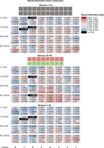
Figure 4 (A–C) Stimulus-dependent distribution of linear MI across the array.

Notes: (A) Difference in linear MI for high-γ-band LFP power due to stimulation with luminance contrast – chromatic contrast stimuli. Red indicates that electrodes in the thin stripe exhibited greater MI_linear in response to the chromatic stimulus set. (B) Difference in MI_linear for high-γ-band LFP power in response to red/gray – green/gray chromatic contrast stimuli. Red indicates electrodes with more MI_linear about green/gray stimuli. (C) Difference in MI_linear for high-γ-band LFP power in response to stimulation with luminance contrast gratings of two different spatial frequencies (0.5–2.0 cycles/degree). Red in the type II interstripe indicates this stripe exhibited MI_linear about the higher-spatial-frequency gratings, whereas green in the type I interstripe indicates greater information about the lower-spatial-frequency gratings.
Abbreviations: MI, mutual information; LFP, local field potential; sf, spatial frequency; diff, difference.

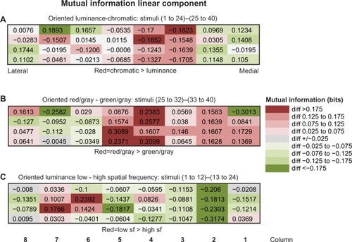
Figure 5 (A and B) Noise correlations as a function of single-unit cortical separation.

Notes: (A) The relationship between noise correlation (correlated variability) and single-unit-pair cortical separation was found to depend on the orientation preferences of the unit pairs. Unit pairs with preferred orientations differing by less than 60° showed the expected decrease in noise correlations with increased distance (blue). Nearby neurons showed high noise correlations (~0.2), while pairs separated by 2 mm had low correlations (~0.05). A similar pattern was observed for neuron pairs spanning the two interstripes with orientation differences >60° (red). Surprisingly, other neuron pairs with orientation differences >60° showed an increase in noise correlations with distance. (B) Relationship between unit noise correlations and cortical separation during stimulation with isoluminant hue patches. Noise correlations were greatest for units recorded at the same electrode (~0.3) and decreased rapidly with cortical separation.

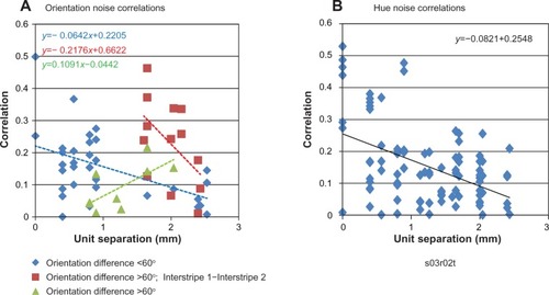
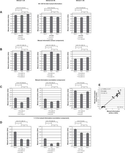
Figure 6 (A and B) Mutual information (MI) varies with reference-electrode position.

Notes: (A) Linear component of MI derived from the power of high-γ-frequency (60–120 Hz) local field potentials (LFPs) from the luminance, chromatic, and total stimulus sets. Lighter shades of blue indicate greater MI_linear. (B) M_Itotal from high-γ-frequency LFP power determined by calculating the MI due to correlations arising from the correlations with the reference electrode (black outline in each array) and adding those to the MI_linear. The distribution of MI_total varied systematically with the position shift on the reference electrode. Interactions in the immediate vicinity of the reference electrode tended to produce the smallest MI_correlation, and thus smallest increases above MI_linear, whereas more distant electrodes demonstrated more substantial increases in MI_total, due to MI_correlation with the reference site. Furthermore, the pattern of increases in MI_total was not confined to a single array column, but rather seemed to reflect the pattern of interactions with each separate stripe compartment.

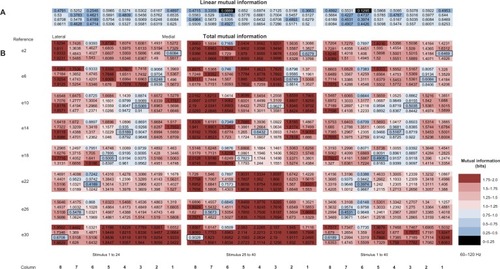
Figure 7 (A–D) Distribution of mutual information (MI) components due to interactions with the reference electrode.

Notes: (A) Representation of MI_total in each microelectrode-array column and stripe compartment as a function of reference-electrode position and stimulus epoch. Each data point reflects the mean (± standard error of mean) arising from electrodes assigned to each stripe compartment as a function of reference-electrode position; 60–120 Hz. (B) Representation of MIl_inear due to interactions with the reference electrode; 60–120 Hz. (C) Representation of MI_correlation due to reference-electrode position. In general, MI_correlation was minimized when the reference electrode was located within the corresponding stripe borders; 60–120 Hz. (D) Compact representation of MI_correlation due to reference-electrode position, 1–13 Hz local field potential frequency band. In general, the distribution of MI_correlation in the 1–13 Hz band was similar to that observed within the 60–120 Hz high-γ-frequency band. The pale aqua rectangle indicates the approximate position of the thin stripe.

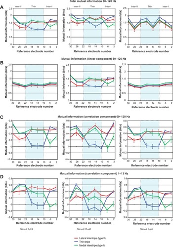
Figure 8 (A–D) Mutual information (MI) in cytochrome oxidase (CO) stripes varied systematically due to interstripe interactions.

Notes: (A) MI_total in each CO stripe was modified by interactions with each “reference” stripe in the achromatic (stimuli 1–24), chromatic (stimuli 25–40), and full-stimulus (stimuli 1–40) sets (columns). In each stimulus condition, MI_total is plotted for each stripe (interstripe II, thin, and interstripe I) as a function of the reference stripe, which provided the specific stripe–stripe interactions. For each triplet in each stimulus condition, MI_total varied significantly across stripes (Kruskal–Wallis test). Within each reference-stripe condition, nonparametric tests were used to determine the significance of differences in MI_total between stripes (Wilcoxon, uncorrected for multiple tests). (B) MI_linear was significantly different across stripes in each reference stripe condition for the achromatic, chromatic, and full-stimulus conditions. Within each reference stripe condition, nonparametric tests were used to determine the significance of differences in MI_linear between stripes (Wilcoxon, uncorrected for multiple tests). In most reference-stripe and stimulus conditions, MI_linear was observed to vary significantly between stripe pairs. However, in several instances, MI_linear did not distinguish the CO compartments. For example, in the achromatic stimulus condition using interstripe I as reference, all of the pair-wise comparisons between stripes failed to reach statistical significance. Similarly, in the chromatic stimulus condition, with the thin stripe as reference, the MI_linear observed in the type II interstripe was indistinguishable from the thin stripe (P>0.147) and type I interstripe (P>0.052). (C) MI_correlation varied significantly across CO stripes in each stimulus condition and each reference-stripe condition (Kruskal–Wallis). Pair-wise comparisons of MI_correlation within each stimulus and reference-stripe condition revealed that MI_correlation was minimized in each stripe when that stripe served as the reference stripe. (D) The 1–13 Hz band of MI_linear varied significantly across stripes in each stimulus and reference-stripe condition (Kruskal–Wallis). Similar to MI_correlation in the high-γ-band, pair-wise comparisons between stripes in each reference-stripe condition revealed that MI_correlation was minimal within each stripe that serves as the reference (Wilcoxon). This effect was most obvious within the chromatic stimulus condition, where MI_correlation was found to be negative for the thin stripe and interstripe I when they served as the reference stripe.

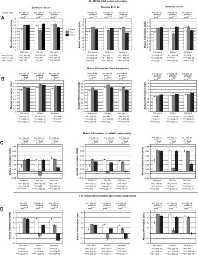
Figure 9 (A–E) Mutual information (MI) due to interstripe interactions.

Notes: (A) MI_total from the high-γ-band varied significantly across stripes in each stimulus condition. In these and all other plots in this figure, the interstripe interactions under the different reference-stripe conditions have been reanalyzed to reflect the full impact of interactions between stripes. Pair-wise comparisons between stripes in each stimulus condition revealed that MI_total was significantly different between type II and type I interstripes, but thin stripes were indistinguishable from type II interstripes in each stimulus condition. (B) MI_linear varied significantly across stripes in each stimulus condition. In both the achromatic and chromatic stimulus conditions, MI_linear was greatest within the thin stripe. However, in the full-stimulus condition, MI_linear was maximal in the type I interstripe. (C) MI_correlation varied significantly across stripes in each stimulus condition. Pair-wise comparisons between stripes revealed that MI_correlation was smallest in the achromatic and full-stimulus conditions, and smaller than MI_correlation within interstripe II in the chromatic condition. (D) The 1–13 Hz MI_correlation varied significantly between stripes in all stimulus conditions. Unlike the high-γ-band MI_correlation, pair-wise comparisons revealed that 1–13 Hz MI_correlation was greatest in the type II interstripe in each stimulus condition. (E) Reproducibility of MI estimates across trials. Plot of correlation of MI_total, MI_linear, and MI_correlation from two independent repetitions of this stimulus set, separated by 2 hours, within a single recording session. The correlation was robust (R²=0.961) and highly significant (P<4.44 × 10⁻¹⁹).