Distinct patterns of corticogeniculate feedback to different layers of the lateral geniculate nucleus

Figures & data

Figure 1 Photomicrographs of two iontophoretic BDA injection sites.

Notes: (A) Coronal section through the dorsal bank of V1. (B) The transported label in a parasagittal section through the LGN from the same case. The injections were centered in cortical layer 6 and confined to the infragranular layers of V1 (eg, layer 4 and 5). Here, we used cortical layer designations as follows with Brodmann’s¹⁹ terminology in parenthesis where it differs: 3C (4B), 4α (4Cα), 4β (4Cβ). The rationale for this choice is given in Casagrande and Kaas.¹⁸ The labeled axons in the LGN form two columns (arrows) that correspond to the pair of injections in layer 6 of V1. Numerals in LGN indicate different K layers. Scale bar =500 μm for (A) and (B).
Abbreviations: BDA, biotinylated dextran; D, dorsal; K, koniocellular; L, lateral; LGN, lateral geniculate nucleus; Mc, contralateral magnocellular; Mi, ipsilateral magnocellular; P, posterior; Pc, contralateral parvocellular; Pi, ipsilateral parvocellular; V1, primary visual cortex.

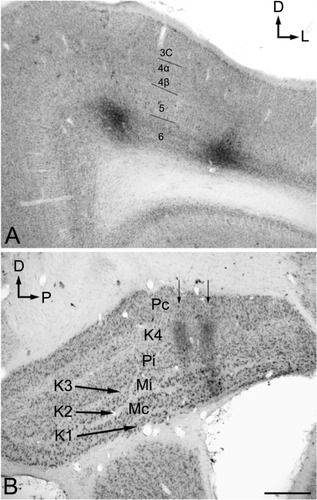
Figure 2 High power photomicrographs of boutons labeled after injections into V1 that filled a small number of layer 6 cells.

Notes: (A) LGN, (B) TRN, and (C) pulvinar. Terminations in the TRN are likely collaterals of axons that terminate in the adjacent LGN, but the pulvinar axons arise from separate cells. Arrowheads in (A) point to dendrites of a retrogradely filled cell in the LGN. Arrows in (A) and (B) compare bouton sizes on corticothalamic axons in the LGN and TRN, respectively. Scale bar =10 μm.
Abbreviations: LGN, lateral geniculate nucleus; TRN, thalamic reticular nucleus.

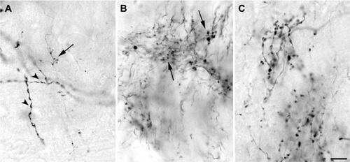
Figure 3 High power photomicrographs of axons within the LGN.

Notes: (A) P, (B) K, and (C) M layers. There was no qualitative difference in axon caliber or bouton size that correlated with LGN layer type. Corticogeniculate axons, arrow in (C), were much finer than geniculate relay cell dendrites (arrowheads). Scale bar =10 μm.
Abbreviations: K, koniocellular; LGN, lateral geniculate nucleus; M, magnocellular; P, parvocellular.

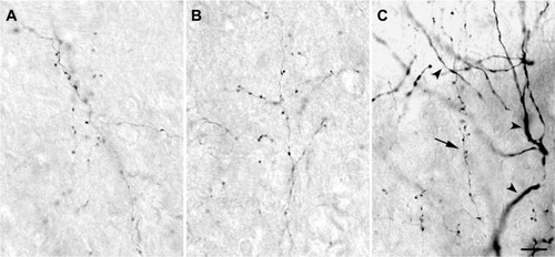
Figure 4 Reconstructions showing corticogeniculate axon branching patterns in the M LGN layers.

Notes: (A) An axon that innervated the M layer receiving input from the contralateral eye with branches in adjacent K layers K1 and K2. (B) Reconstruction of an axon that innervated both M layers with branches in K1, K2, and K3. Scale bars =50 μm.
Abbreviations: K, koniocellular; LGN, lateral geniculate nucleus; M, magnocellular; Mc, contralateral magnocellular; Mi, ipsilateral magnocellular; Pc, contralateral parvocellular; Pi, ipsilateral parvocellular.

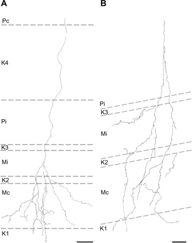
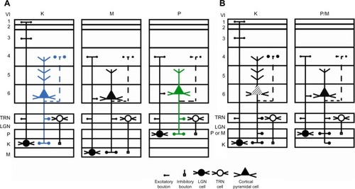
Figure 5 Schematic diagrams summarizing the branching patterns of corticogeniculate axons.

Notes: Corticogeniculate axons reconstructed in the (A) M layers (n=10), (B) P layers (n=9), and (C) K layers (n=2). The number and length of bars are not intended to represent exact branch length, but give a general idea of branch density within each LGN layer. The axons marked with a ★ are also shown in Figure 4 (A), Figure 6 (B) and Figure 7 (C). Branches that terminate in K layers for every axon are indicated in red.
Abbreviations: K, koniocellular; ${\mathrm{K}}_{\mathrm{i}}^{\mathrm{c}}$, koniocellular contralateral and ipsilateral portions of layer; LGN, lateral geniculate nucleus; M, magnocellular; Mc, contralateral magnocellular; Mi, ipsilateral magnocellular; P, parvocellular; Pc, contralateral parvocellular; Pi, ipsilateral parvocellular.

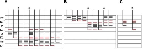
Figure 6 Reconstructions showing corticogeniculate axon branching patterns in the P layers.

Notes: (A) An axon that innervated the ipsilateral P layer with some branches in the ipsilateral portion of K4. (B) An axon that innervates both P layers along with all of K4. Scale bars =50 μm.
Abbreviations: K, koniocellular; P, parvocellular; Pc, contralateral parvocellular; Pi, ipsilateral parvocellular.

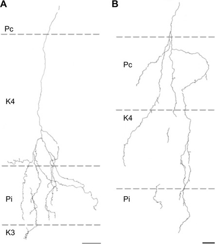
Figure 7 Reconstruction of a corticogeniculate axon that innervated primarily K layers with branches in K4 and K3 as well as the ipsilateral P layer.

Note: Scale bar =50 μm.
Abbreviations: K, koniocellular; P, parvocellular; Pc, contralateral parvocellular; Pi, ipsilateral parvocellular.

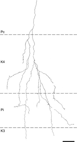
Figure 8 Electron micrographs of BDA-labeled corticogeniculate terminals in the LGN.

Notes: Labeled corticogeniculate terminals contain a dense black reaction product. Gold particles indicate the presence of GABA. (A) Labeled corticogeniculate terminal in a K layer making a synapse (arrow) onto an unlabeled (presumed glutamatergic) relay cell dendrite. (B) Labeled corticogeniculate terminal in an M layer with a synapse (arrow) on an unlabeled (presumed glutamatergic) dendrite, which received additional input from unlabeled terminal (on the right). (C) Labeled corticogeniculate terminal in a P layer with a synapse (arrow) on an unlabeled (presumed glutamatergic) dendrite. (D) An example of an infrequent corticogeniculate axon with a synapse (arrow) on a small GABAergic dendrite (GABA) in a P layer. Scale bar =0.2 μm.
Abbreviations: BDA, biotinylated dextran; K, koniocellular; LGN, lateral geniculate nucleus; M, magnocellular; P, parvocellular; GABA, γ-Aminobutyric acid.

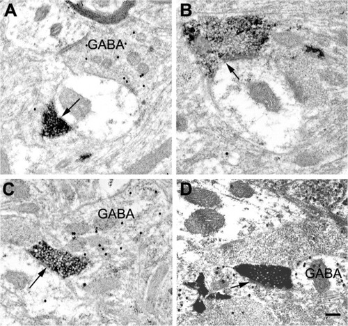
Figure 9 Photomicrographs of an iontophoretic injection in the LGN and the same section Nissl stained to reveal the LGN layers.

Notes: (A) Iontophoretic injection in the LGN. (B) The same section Nissl stained to reveal the LGN layers. The fluorescent injection site (arrow in [A] and green in [B]) is centered in the contralateral M layer. Scale bar =500 μm.
Abbreviations: A, anterior; D, dorsal; K, koniocellular; LGN, lateral geniculate nucleus; M, magnocellular; Mc, contralateral magnocellular; Mi, ipsilateral magnocellular; Pc, contralateral parvocellular; Pi, ipsilateral parvocellular.

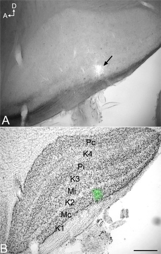
Figure 10 Photomicrographs of an intracellularly filled cell in layer 6 of the primary visual cortex.

Notes: (A) The cell body, many basal dendrites, and most of the apical dendrite are visible in this section. Scale bar =50 μm. (B and C) Higher power photomicrographs show well filled and easily distinguishable spines indicating that the filling was very complete. Scale bar =10 μm.

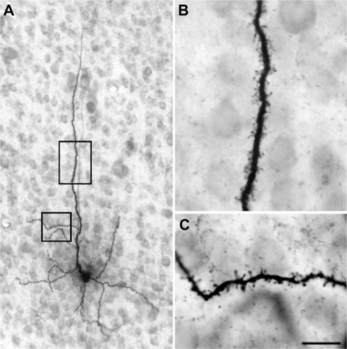
Figure 11 Reconstruction of a corticogeniculate cell that was labeled following an injection into the M layers of the LGN.

Notes: Most of this cell’s dendrites were restricted to layer 6. Only the apical dendrite extended beyond the layer 5/6 boundary. The inset shows the location of the injection site in the LGN. Scale bar =50 μm (500 μm in the inset).
Abbreviations: A, anterior; D, dorsal; K, koniocellular; LGN, lateral geniculate nucleus; M, magnocellular; P, parvocellular; WM, white matter.

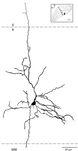
Figure 12 Reconstruction of a corticogeniculate cell that was labeled following an injection into the P layers of the LGN.

Notes: The basal dendrites were arranged radially around the soma and were confined to layer 6. The apical dendrite extended up to the layer 4/5 boundary with branches in the upper part of layer 6 and a few sparse branches in layer 5. Scale bar =50 μm (500 μm in the inset).
Abbreviations: A, anterior; D, dorsal; K, koniocellular; LGN, lateral geniculate nucleus; M, magnocellular; P, parvocellular; WM, white matter.

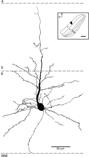
Figure 13 Reconstruction of a corticogeniculate cell that was labeled following an injection into the K layers of the LGN.

Notes: The basal dendrites were arranged radially around the soma and were confined to layer 6. The apical dendrite extended into layer 4 with branches in the upper part of layer 6, layer 5, and layer 4. Scale bar =50 μm (500 μm in the inset).
Abbreviations: A, anterior; D, dorsal; K, koniocellular; LGN, lateral geniculate nucleus; M, magnocellular; P, parvocellular.

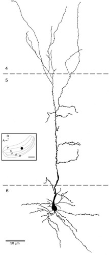
Figure 14 Schematic diagram summarizing the dendritic arborizations of all filled and reconstructed cells.

Notes: Filled and reconstructed cells projecting to (A) an M LGN layer, (B) a P LGN layer, or (C) K4. The number and length of the dendritic branches are not intended to represent the exact length, but to give a general idea of branch density within each cortical layer. Cells colored red are those with spines in cortical layer 4. Cells indicated by a ★ is also shown in Figure 11 (A), Figure 12 (B) and Figure 13 (C).
Abbreviations: K, koniocellular; LGN, lateral geniculate nucleus; M, magnocellular; P, parvocellular.

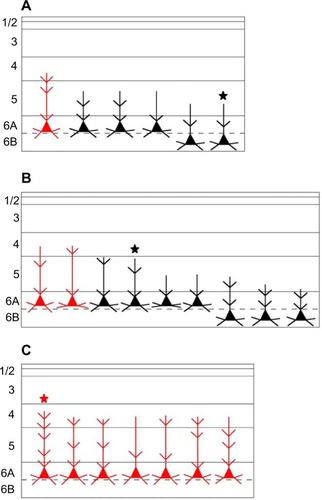
Figure 15 Distributions of corticogeniculate cell dendrites.

Notes: (A) Shows the distribution of dendrites per cortical layer. The majority of dendrites were located within layer 6. (B) Shows the percentage of dendritic length in each cortical layer for each corticogeniculate cell class. The distributions of dendrites is similar for M and P corticogeniculate cells and distinct from K corticogeniculate cells. (C) Shows the distribution of dendrites broken down by the LGN layer to which they project. K-projecting cells have a more even distribution of dendrites across layers 4, 5, and 6 with significantly more dendritic arbor in layer 4, while M- and P-projecting cells have the majority of their dendrites in layer 6.
Abbreviations: K, koniocellular; LGN, lateral geniculate nucleus; M, magnocellular; P, parvocellular.

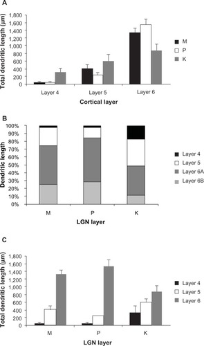
Figure 16 Schematic diagram summarizing two interpretations of the main corticogeniculate pathways in primates.

Notes: (A) Shows the three main pathways in the macaque monkey. The K pathway (blue) is shown on the left and represents only the blue on-portion of the K pathway based on a combination of anatomical and physiological data.¹² The M pathway (black) is in the center and the P pathway (green) is on the right. (B) Compares the M and P pathways in bush babies and owl monkeys¹⁴ with the K pathway based primarily on anatomical data. The K pathway (striped) is shown on the left and the P/M pathways are shown on the right. Symbols below the figure identify different features. Arabic numerals refer to the V1 layers. Dotted lines indicate data either not shown or not part of this study but demonstrated in other studies.
Abbreviations: K, koniocellular; LGN, lateral geniculate nucleus; M, magnocellular; P, parvocellular; TRN, thalamic reticular nucleus; V1, primary visual cortex.

BrodmannKLocalization in the Cerebral CortexLeipzigJohann Ambrosius Barth1909

 Google Scholar

CasagrandeVAKaasJHThe afferant, intrinsic, and efferent connections of primary visual cortex in primatesPetersARocklandKSPrimary Visual Cortex of Primates Cerebral Cortex10New YorkPlenum1994201259

 Google Scholar

BriggsFUsreyWMParallel processing in the corticogeniculate pathway of the macaque monkeyNeuron200962113514619376073

 PubMed Web of Science ®Google Scholar

IchidaJMCasagrandeVAOrganization of the feedback pathway from striate cortex (V1) to the lateral geniculate nucleus (LGN) in the owl monkey (Aotus trivirgatus)J Comp Neurol2002454327228312442318

 PubMed Web of Science ®Google Scholar