Figures & data
Figure 1 Morbidity rate of TB and decomposed trend, seasonality and random pattern with the multiplicative seasonal decomposition technique during January 2004 to December 2016 in Qinghai Province. (A) Time plot for the TB morbidity rate series; (B) Trend pattern for the TB morbidity rate series; (C) Seasonal pattern for the TB morbidity rate series; (D) Error component for the TB morbidity rate series.
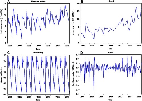
Table 1 Information Criteria Values of the Six Candidate SARIMA Models
Table 2 Resulting Parameter Estimates and Their Statistical Tests of the Best-Fitting SARIMA(2,0,2)(1,1,0)12 Model
Table 3 Ljung–Box Q Statistics for the Residual Series Yielded by the Best-Performing Three Techniques at Various Lags
Table 4 ARCH Effects for the Actual TB Incidence Rate and Residual Series Yielded by the Best-Performing Three Techniques at Various Lags
Table 5 Forecasts Between January 2016 and December 2016 Achieved by Adopting the Best-Fitting Three Techniques
Figure 2 Test statistics for the residual series of TB incidence rate from the SARIMA(2,0,2)(1,1,0)12 model. (A) Standardized residual series; (B) Autocorrelogram (ACF) for the residual series; (C) Partial autocorrelogram (PACF) for the residual series; (D) P values for Ljung–Box statistic. It was seen that none of correlation coefficients except that at lag 31 in the PACF graph exceeded the estimated 95% confidence intervals. For this point at lag 31, it is reasonable as the higher lag is easily outside the limits by chance. All these above intimated that the identified SARIMA technique seems adequate and applicable in describing the dynamic dependence of the data.
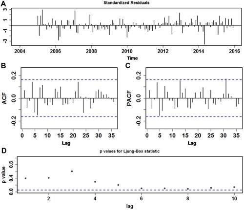
Table 6 Comparisons of the Mimic and Predictive Performance Measures Among the Best-Performing Three Models
Figure 3 Diagnostic tests for the residual series of TB morbidity rate from the NNNAR(7,1,4)12 technique. (A) Standardized residual series; (B) Autocorrelation function (ACF) plot for the residual series; (C) Partial autocorrelation function (PACF) plot for the residual series; (D) Q-statistic P-values. As seen, the sample ACF and PACF of residuals revealed no significant serial correlations suggesting that the chosen NNNAR method is suitable for capturing the serial dependence of the data.
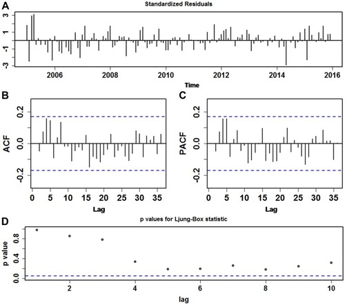
Figure 4 Tests of goodness of fit for the error series of TB morbidity rate from the SARIMA-NNNAR(3,1,7)12combined method. (A) Standardized residual series; (B) Autocorrelation function (ACF) plot for the residual series; (C) Partial autocorrelation function (PACF) plot for the residual series; (D) Q-statistic P-values. As presented, there were no sample ACF and PACF falling approximately out of the 95% uncertainty bounds other than that at lag 10 in the ACF and PACF graphs. These manifested its adequacy and suitability of this data-driven hybrid model for the data.
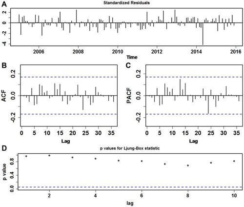
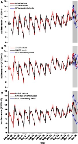
Figure 5 Resulting comparisons of the in-sample mimics and out-of-sample projections using the preferred three models. A projection for the hold-out 12 months’ data was as the shaded area. Overall, it was seen that the simulations and forecasts (black solid line) with the advanced data-driven SARIMA-NNNAR combined model provided a better approximation to the actual morbidity rate (red solid line) than both the SARIMA and NNNAR models. (A) SARIMA model; (B) NNNAR model; (C) SARIMA-NNNAR model.