Secular Seasonality and Trend Forecasting of Tuberculosis Incidence Rate in China Using the Advanced Error-Trend-Seasonal Framework

Figures & data

Table 1 The 30 Alterative ETS Methods Associated with Various Combinations of Trend, Seasonality and Error

Trend Pattern	Seasonal Pattern
	N (None)	A (Additive)	M (Multiplicative)
ETS Framework with Additive Form
N (None)	N,A,N	N,A,A	N,A,M
A (Additive)	A,A,N	A,A,A	A,A,M
AD (Additive damped)	AD,A,N	AD,A,A	AD,A,M
M (Multiplicative)	M,A,N	M,A,A	M,A,M
MD(Multiplicative damped)	MD,A,N	MD,A,A	MD,A,M
ETS Framework with Multiplicative Form
N (None)	N,M,N	N,M,A	N,M,M
A (Additive)	A,M,N	A,M,A	A,M,M
AD (Additive damped)	AD,M,N	AD,M,A	AD,M,M
M (Multiplicative)	M,M,N	M,M,A	M,M,M
MD(Multiplicative damped)	MD,M,N	MD,M,A	MD,M,M

Abbreviation: ETS, error-trend-seasonal.

Figure 1 Joinpoint regression displaying the TB epidemic trends over the period 1997–2035. *Showed that the annual percent change (APC) is significantly different from zero at the significance level.

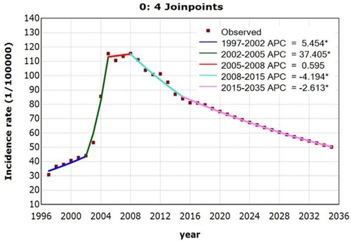
Figure 2 Time-series plot for the monthly TB incidence in China from January 1997 to August 2019 and the seasonal decomposition consisting of different components of the TB series with the STL method. (A) TB incidence time series; (B) trend component; (C) seasonal component; (D) irregular component.

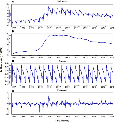
Figure 3 Monthly TB incidence plot averaged by season.

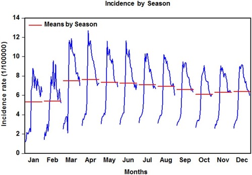
Table 2 The Best-Performing SARIMA Models Obtained from Various Training Sets and Goodness of Fit Tests for Their Parameters

Parameters	Coefficients	S.E.	t	P	Stationary R^2	R^2	Normalized BIC	Ljung-Box
								Statistics	P
SARIMA(0,1,(1,10))(0,1,1)12 Model Yielded Based on the Observations from January 1997 to August 2018
MA1	0.692	0.044	15.705	<0.001	0.617	0.931	−0.753	13.851	0.537
MA10	−0.201	0.045	−4.439	<0.001
SMA1	0.764	0.049	15.519	<0.001
SARIMA(0,1,(1,10))(0,1,1)12 Model Yielded Based on the Observations from January 1997 to August 2017
MA1	0.691	0.045	15.282	<0.001	0.612	0.932	−0.720	12.186	0.665
MA10	−0.209	0.046	−4.503	0.001
SMA1	0.776	0.050	15.494	<0.001
SARIMA(0,1,1)(1,1,1)12 Model Yielded Based on the Observations from January 1997 to August 2016
MA1	−0.622	0.052	−11.961	<0.001	0.613	0.935	−0.644	21.845	0.239
SAR1	0.207	0.123	1.683	0.047
SMA1	−0.798	0.105	−7.600	<0.001
SARIMA(0,1,1)(1,1,1)12 Model Yielded Based on the Observations from January 1997 to August 2015
MA1	−0.623	0.053	−11.755	<0.001	0.612	0.935	−0.634	21.020	0.278
SAR1	0.226	0.128	1.766	0.039
SMA1	−0.814	0.111	−7.333	<0.001
SARIMA(0,1,1)(0,1,1)12 Model Yielded Based on the Observations from January 1997 to August 2013
MA1	0.629	0.060	10.528	<0.001	0.591	0.931	−0.510	21.800	0.150
SMA1	0.730	0.063	11.563	<0.001
SARIMA(0,1,1)(0,1,1)12 Model Yielded Based on the Observations from January 1997 to August 2011
MA1	0.609	0.065	9.311	<0.001	0.586	0.937	−0.495	22.785	0.120
SMA1	0.748	0.069	10.775	<0.001
SARIMA(0,1,1)(0,1,1)12 Model Yielded Based on the Observations from January 1997 to August 2010
MA1	0.606	0.068	8.887	<0.001	0.586	0.936	−0.444	20.979	0.179
SMA1	0.767	0.075	10.261	<0.001
SARIMA(0,1,1)(0,1,1)12 Model Yielded Based on the Observations from January 1997 to August 2008
MA1	0.588	0.075	7.835	<0.001	0.527	0.937	−0.455	17.500	0.354
SMA1	0.691	0.089	7.797	<0.001

Abbreviations: SARIMA, seasonal autoregressive integrated moving average; AR1, autoregressive, lag1; MA1, moving average, lag1; MA10, moving average, lag10; SAR1, seasonal autoregressive, lag1; SMA1, seasonal moving average, lag1; SE, standard error.

Figure 4 Goodness of fit test for the residuals generated by the SARIMA(0,1,(1,10))(0,1,1)₁₂ approach established with the training data from January 1997 to August 2018. (A) Autocorrelation function (ACF); (B) partial autocorrelation function (PACF); (C) P values for Ljung–Box statistic. Almost all of correlation coefficients fell into the 95% uncertainty levels and all P values at different lags were greater than the significance level of 0.05, indicating that this approach showed a good adequacy for this series.

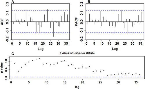
Figure 5 Comparative time series plots measuring the approximations to the hold-out data on different-step-ahead predictions using the SARIMA and ETS methods. (A) 12 data ahead forecasts; (B) 24 data ahead forecasts; (C) 36 data ahead forecasts; (D) 48 data ahead forecasts; (E) 72 data ahead forecasts; (F) 96 data ahead forecasts; (G) 108 data ahead forecasts; (H) 132 data ahead forecasts. In these plots, the shaded areas displayed the predictive results using the SARIMA and ETS models, suggesting that the ETS methods captured the dependent structures well, particularly for the long-term forecasting time steps.

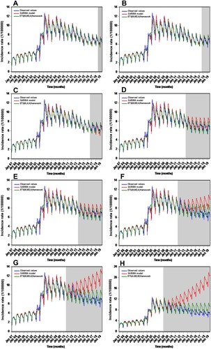
Table 3 The Best-Performing ETS Models Obtained from Various Training Sets and Goodness of Fit Tests for Their Parameters

Parameters	Compact LL	LL	AIC	BIC	HQ	AMSE
ETS(M,MD,A) Approach Erected with the Observations from January 1997 to August 2018
α=0.184	−590.972	−237.007	1215.944	1276.475	1240.278	0.495
β=0.046
γ=0.173
δ=0.950
ETS(M,MD,A) Approach Erected with the Observations from January 1997 to August 2017
α=0.193	−559.392	−227.623	1152.783	1212.512	1176.828	0.518
β=0.045
γ=0.149
δ=0.951
ETS(M,A,A) Approach Erected with the Observations from January 1997 to August 2016
α=0.219	−528.885	−219.022	1089.770	1145.191	1112.110	0.540
β=0.044
γ=0.150
δ=0.000
ETS(M,A,A) Approach Erected with the Observations from January 1997 to August 2015
α=0.216	−498.979	−210.717	1029.957	1084.544	1051.991	0.562
β=0.045
γ=0.147
δ=0.000
ETS(M,MD,A) Approach Erected with the Observations from January 1997 to August 2013
α=0.162	−434.865	−188.821	903.730	959.801	926.421	0.594
β=0.052
γ=0.147
δ=0.950
ETS(M,MD,A) Approach Erected with the Observations from January 1997 to August 2011
α=0.151	−365.918	−160.649	765.836	819.734	787.697	0.605
β=0.054
γ=0.161
δ=0.952
ETS(M,MD,A) Approach Erected with the Observations from January 1997 to August 2010
α=0.142	−334.855	−149.372	703.711	756.409	725.104	0.633
β=0.055
γ=0.166
δ=0.951
ETS(A,MD,M) Approach Erected with the Observations from January 1997 to August 2008
α=0.477	−273.287	−126.023	580.574	630.582	600.896	0.492
β=0.036
γ=0.000
δ=0.929

Abbreviations: ETS, error-trend-seasonal; LL, likelihood; AIC, Akaike information criterion, BIC, Bayesian information criterion; HQ, Hannan–Quinn criterion; AMSE, average mean square error.

Table 4 Comparative Results of the Performances Between the Best-Undertaking SARIMA Methods and the Best-Undertaking ETS Methods on the Different Training and Testing Sets

Models	Training Part				Testing Part
	MAD	MAPE	RMSE	MER	MAD	MAPE	RMSE	MER
260 Training Data from January 1997 to August 2018					12 data ahead
ETS(M,MD,A)	0.412	0.065	0.658	0.062	0.267	0.041	0.344	0.041
SARIMA(0,1,(1,10))(0,1,1)12	0.445	0.069	0.659	0.074	0.278	0.043	0.333	0.043
248 Training Data from January 1997 to August 2017					24 data ahead
ETS(M,MD,A)	0.420	0.066	0.670	0.063	0.383	0.059	0.490	0.058
SARIMA(0,1,(1,10))(0,1,1)12	0.453	0.071	0.669	0.075	0.440	0.068	0.531	0.067
236 Training Data from January 1997 to August 2016					36 data ahead
ETS(M,A,A)	0.425	0.067	0.681	0.064	0.317	0.048	0.441	0.048
SARIMA(0,1,1)(1,1,1)12	0.432	0.068	0.683	0.072	0.432	0.065	0.542	0.065
224 Training Data from January 1997 to August 2015					48 data ahead
ETS(M,A,A)	0.433	0.069	0.695	0.065	0.380	0.056	0.487	0.057
SARIMA(0,1,1)(1,1,1)12	0.443	0.070	0.698	0.074	0.314	0.047	0.428	0.047
200 Training Data from January 1997 to August 2013					72 data ahead
ETS(M,MD,A)	0.446	0.072	0.719	0.068	0.360	0.053	0.480	0.052
SARIMA(0,1,1)(0,1,1)12	0.495	0.078	0.750	0.082	0.745	0.109	0.842	0.108
176 Training Data from January 1997 to August 2011					96 data ahead
ETS(M,MD,A)	0.438	0.073	0.723	0.069	0.665	0.093	0.807	0.092
SARIMA(0,1,1)(0,1,1)12	0.493	0.080	0.752	0.082	1.591	0.231	1.900	0.219
164 Training Data from January 1997 to August 2010					108 data ahead
ETS(M,MD,A)	0.448	0.076	0.741	0.072	0.699	0.097	0.857	0.095
SARIMA(0,1,1)(0,1,1)12	0.503	0.083	0.769	0.084	2.772	0.400	3.287	0.375
140 Training Data from January 1997 to August 2008					132 data ahead
ETS(A,MD,M)	0.396	0.092	0.595	0.070	1.207	0.168	1.553	0.176
SARIMA(0,1,1)(0,1,1)12	0.472	0.085	0.761	0.079	6.099	0.867	7.364	0.890

Abbreviations: SARIMA, seasonal autoregressive integrated moving average; ETS, error-trend-seasonal; MAD, mean absolute deviation; MAPE, mean absolute percentage error; RMSE, root mean squared error; MER, mean error rate.

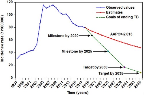
Figure 6 Annual TB incidence projections up to 2035 using the ETS(M,M,M) method based on the entire dataset. As illustrated, albeit the TB incidence continued to display a declined trend at 2.613% per year in China, it showed major challenges ahead to achieve the WHO’s milestones and goals.