Figures & data
Figure 1 Time series displaying the HFMD incidence from January 2009 to December 2019 and the decomposed trend, seasonal, and random traits using the classical multiplicative decomposition method.
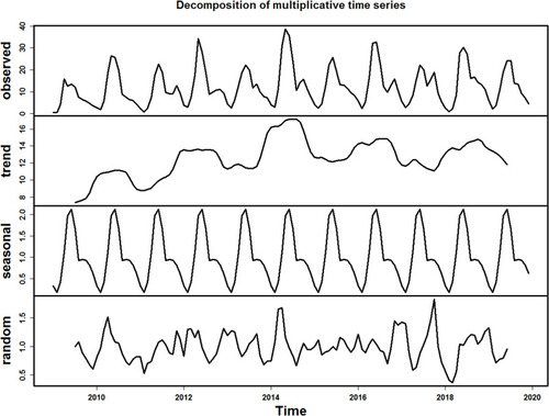
Table 1 The Identified Eight Possible SARIMA Methods and Their Corresponding Information Criteria
Table 2 Statistical Test of the Estimated Parameters for the Optimal SARIMA (1,0,1)(0,1,1)12 Method
Table 3 Box-Ljung Q and LM Tests of the Residual Series from the Optimal SARIMA (1,0,1)(0,1,1)12 and TBATS(0.062, {1,3}, 0.86, {<12,4>}) Methods
Figure 2 Diagnostic checking for the residual series from the best SARIMA (1,0,1)(0,1,1)12 method. (A) Correlogram of the sample autocorrelation function (ACF); (B) Correlogram of the sample partial autocorrelation function (PACF); (C) p values for the Ljung-Box test. The plot above showed that almost all the sample autocorrelations for the residual series fail to touch the significance bounds apart from the one at lag 25 (which is also reasonable as higher-order autocorrelation may exceed the 95% significance bounds by chance alone) and p values at different lags are greater than 0.05 under the Ljung-Box statistic, suggesting that there is little evidence of non-zero autocorrelations in the residual series at various lags.
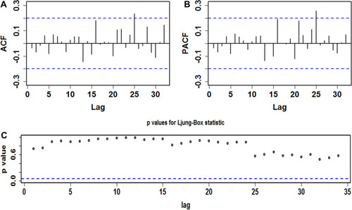
Figure 3 Diagnostic checking for the residual series from the best TBATS (0.062, {1,3}, 0.86, {<12,4>}) method. (A) Correlogram of the sample autocorrelation function (ACF); (B) Correlogram of the sample partial autocorrelation function (PACF); (C) p values for the Ljung-Box test. The plot above showed that almost all the sample autocorrelations for the residual series fail to touch the significance bounds and p values at different lags are greater than 0.05 under the Ljung-Box statistic, suggesting that there is little evidence of non-zero autocorrelations in the residual series at various lags.
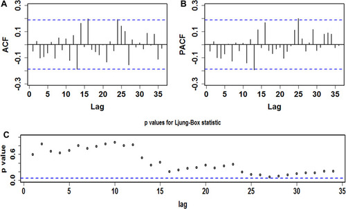
Table 4 Comparisons of the Fitted Parts and the Predicted Parts Between SARIMA Methods and TBATS Methods
Table 5 Forecasts and Their 95% Uncertainty Limits of the HFMD Incidence for the Next 24 Months Based on the TBATS (0.022, {3, 1}, 0.851, {<12, 4>}) Method
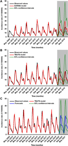
Figure 4 Time series plot showing the in-sample simulation and out-of-sample forecasting using the best SARIMA and TBATS methods. (A) The in-sample fitting and out-of-sample forecasting results using the best SARIMA method; (B) The in-sample fitting and out-of-sample forecasting results using the best TBATS method; (C) The next 24-month projections using the best TBATS method built with the incidence data from January 2009 to December 2019.