Figures & data
Figure 1 Joinpoint regression plot displaying the HFRS epidemiological trends from 1995 to 2020. *Showed that the annual percent change (APC) is statistically significant.
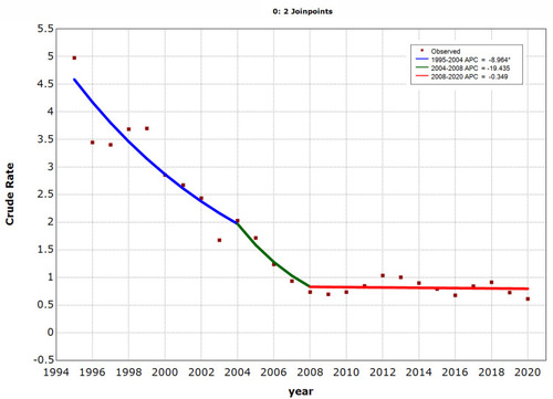
Figure 2 Probability density plot showing the monthly HFRS incidence. As depicted, HFRS showed notable seasonal variation, with a strong peak in November and December, and a weak peak in May and June.
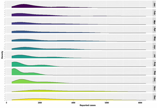
Table 1 The Best-Performing SARIMA Models Obtained on the Various Training Sets and Their Parameter Estimations and Goodness of Fit Tests
Figure 3 Diagnostic test plots for the forecasting errors of the SARIMA model created with the data between 1995 and 2019. (A) Autocorrelation function (ACF) plot, (B) partial autocorrelation function (PACF) plot, and (C) p-values for Ljung-Box statistic. We could see from the sample correlogram that there were little sample ACFs and PACFs touching the significance bounds, except for that at lags 9, 23, and 24, and the p-value was greater than 0.05 under Ljung-Box test statistic. These results meant that the selected SARIMA approach provides an adequate predictive model for the HFRS incidence.
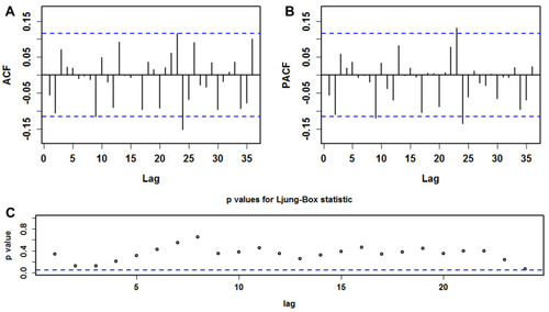
Figure 4 Time series plots showing the forecasted results on different datasets between the SARIMA models and the TBATS models. (A) 12-step ahead forecast, (B) 24-step ahead forecast, (C) 36-step ahead forecast, (D) 60-step ahead forecast, (E) 84-step ahead forecast, and (F) 108-step ahead forecast. The out-of-sample predictions are shown as a shaded area in these plots. It was discovered that the out-of-sample predictions under TBATS approaches agreed better with the observed values over the SARIMA approaches, especially for the long-term out-of-sample predictions.
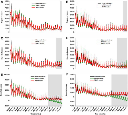
Table 2 Comparisons of the Out-of-Sample Forecasting Powers Between SARIMA Models and TBATS Models
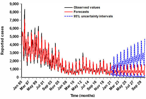
Figure 5 Estimated epidemiological trends and seasonality of HFRS between January 2021 and December 2030 using the best-performing TBATS (0.286, {3,0}, -, {<12,4>}) model.