Figures & data
Figure 1 MC simulation geometry and imaging water phantom.
Notes: (A) MC simulation geometry for pinhole K-shell XRF imaging system and (B) imaging water phantom where four columns are assumed to have different concentrations of either gadolinium (Gd) or gold (Au) nanoparticles. The red arrows indicate the incident fan-beam X-rays. Gd or Au columns of 0.01 wt%, 0.03 wt%, 0.06 wt%, and 0.09 wt% are located left, in, out, and right with respect to the incident direction of X-rays, respectively.
Abbreviations: MC, Monte Carlo; XRF, X-ray fluorescence; Gd, gadolinium; Au, gold; wt, weight.
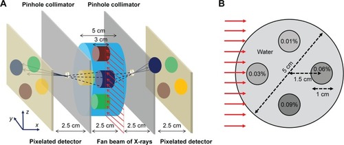
Figure 2 Incident X-ray source spectra for pinhole K-shell XRF imaging for (A) gadolinium and (B) gold.
Abbreviation: XRF, X-ray fluorescence.
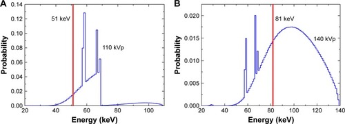
Figure 3 Schematic representation of pinhole XRF imaging system.
Notes: The midplane of the water phantom was divided into 32×32 pixels, each of which had 1.6×1.6 mm2 area. yi is the path length of incident X-rays in the phantom, while xi is the path length of XRF photons of the ith pixel in the phantom.
Abbreviation: XRF, X-ray fluorescence.
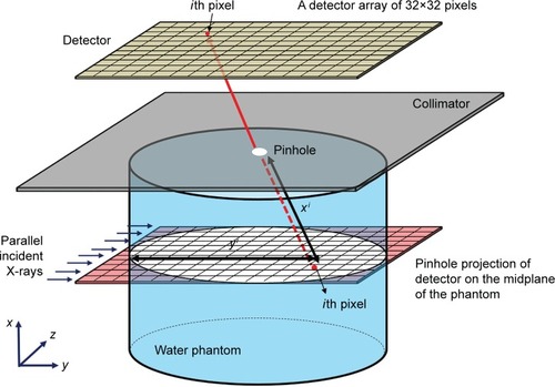
Figure 4 Subtracted and corrected XRF images for Gd.
Notes: (A) Subtracted XRF image between Gd-loaded water phantom and pure water phantom; (B) XRF image of Gd corrected by attenuation and sensitivity for monochromatic 51 keV X-rays; (C) subtracted XRF image between Gd-loaded water phantom and pure water phantom; and (D) XRF image of Gd corrected by attenuation and sensitivity for polychromatic 110 kVp X-rays.
Abbreviations: XRF, X-ray fluorescence; Gd, gadolinium.
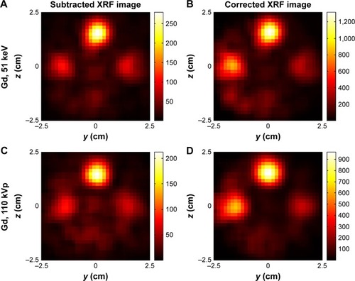
Figure 5 XRF signal intensities and CNR values versus Gd concentrations.
Notes: (A) Linear relationship between Gd concentrations and integrated XRF counts and (B) CNR values in the region of Gd columns for two different X-ray source spectra.
Abbreviations: CNR, contrast-to-noise ratio; XRF, X-ray fluorescence; wt, weight; Gd, gadolinium.
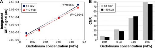
Figure 6 Subtracted and corrected XRF images for Au.
Notes: (A) Subtracted XRF image between Au-loaded water phantom and pure water phantom; (B) XRF image of Au corrected by attenuation and sensitivity for monochromatic 81 keV X-rays; (C) subtracted XRF image between Au-loaded water phantom and pure water phantom; and (D) XRF image of Au corrected by attenuation and sensitivity for polychromatic 140 kVp X-rays.
Abbreviations: XRF, X-ray fluorescence; Au, gold.
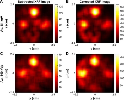
Figure 7 XRF signal intensities and CNR values versus Au concentrations.
Note: (A) Linear relationship between Au concentrations and integrated XRF counts and (B) CNR values in the region of Au columns for two different X-ray source spectra.
Abbreviations: CNR, contrast-to-noise ratio; XRF, X-ray fluorescence; Au, gold.
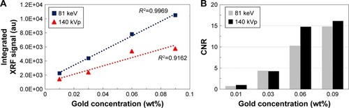
Table 1 Imaging dose of pinhole XRF imaging for four different incident X-ray sources
Figure S1 Schematic of pinhole collimation, where the acceptance angle is 102° and the angle between a point on the midplane of water phantom and the center of pinhole is θ.
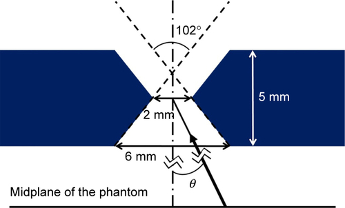
Figure S2 Energy spectrum of Am-241 acquired with the CZT gamma camera.
Abbreviations: CZT, cadmium-zinc-telluride; FWHM, full width at half maximum.
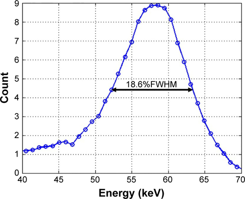
Figure S3 Energy spectra of K-shell XRF and Compton scattered photons from 0.09 wt% Gd column.
Notes: (A) Energy spectra of MC-based 1 keV bin and (B) energy spectra of a degradation with the measured %FWHM. Error bar indicates 68% confidence level.
Abbreviations: FWHM, full width at half maximum; MC, Monte Carlo; XRF, X-ray fluorescence; Gd, gadolinium.
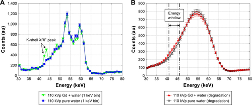
Figure S4 Energy spectra of K-shell XRF and Compton scattered photons from 0.09 wt% Au column.
Notes: (A) Energy spectra of MC-based 1 keV bin and (B) energy spectra of a degradation with the measured %FWHM. Error bar indicates 68% confidence level.
Abbreviations: FWHM, full width at half maximum; MC, Monte Carlo; XRF, X-ray fluorescence; Au, gold; wt, weight.
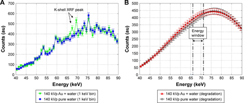
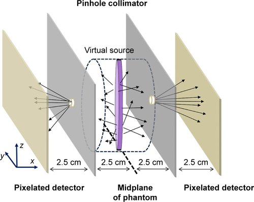
Figure S5 MC simulation model for sensitivity correction.
Notes: The virtual disk source of 5 cm diameter and 5 mm width (purple) in the midplane of water phantom isotropically emits fluorescence-like photons. The arrows describe photons emitting from the virtual source. The photons originating from the center of the source are detected more efficiently than those from the periphery.
Abbreviation: MC, Monte Carlo.