Figures & data
Figure 1 Bright-field microscopic images of the fabricated polymeric tip on the top of a single mode optical fiber dropped into a solution of distilled water.
Notes: (A) The optical fiber image focus plan; (B) the fiber focus plan, and with the laser source turned on for back-scattered signal acquisition after the light input signal interacts with the surrounding media where the micro-lens is dipped.
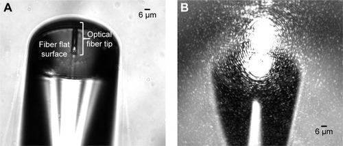
Figure 2 Scheme of the optical setup used to manipulate the fiber tool with the micro-lens on its extremity and acquire the back-scattered signal for nanoparticles detection in aqueous media.
Notes: Adapted from Paiva J et al. Single particle differentiation through 2D optical fiber trapping and Back-Scattered signal statistical analysis: an exploratory approach. Sensors. 2018;18(3):710.Citation21
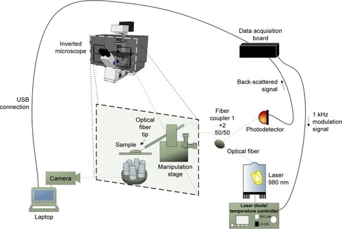
Table 1 Description of the solutions evaluated in this study. Distilled water refractive index (RI)=1.327 (@λ=980 nm); polystyrene RI=1.5731
Figure 3 Scheme explaining all the steps adopted in this study, from signal acquisition to the calculation of a discriminant function to separate the two classes.
Notes: (A) After the back-scattered signal being acquired for each fiber tool location spot and solution, each whole 60 seconds acquisition was filtered using a 500 Hz high-pass filter. (B) Then, each entire acquisition was normalized, by computing the z-score for each signal value. (C) After normalization, each entire signal was segmented into short-term signal portions of 2 seconds. (D) The 2-second signal portions whose values did not comply with the condition |z-score||<5 were removed, to increase the Signal-to-Noise Ratio (SNR). (E) After signal processing, the obtained dataset was composed of 2-second short-term signal portions for each class. (F) A set of 53 parameters based on the time and frequency-domain information was extracted from each 2-second signal portion. (G) Then, two features that gather the most important information provided by the 53 original parameters were generated through the LDA technique. (H) The separation line or discriminant function that better splits the two classes considering a 2D space formed by the two novel features was calculated. At the end of the proposed differentiation problem, the equation of this separation line dictates the class where a sample/set of samples belong, after projecting the 53 features into the two LDA-derived ones. Figure adapted from Workman, C et al. A new non-linear normalization method for reducing variability in DNA microarray experiments. Genome biology, 2012;3(9):research0048-1.Citation49
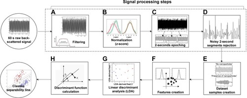
Table 2 Final dataset characterization
Figure 4 Plots of the processed back-scattered signal portions acquired when the fabricated fiber tool was dipped into (Ai) and (Aii) Solution 1, the “blank” solution containing only distilled water; (Bi) Solution 5, a distilled water solution containing 100 nm polystyrene nanoparticles in a concentration of 3.89 µg/mL; and (Bii) Solution 10, with 100 nm polystyrene nanoparticles in a concentration of 1.22E-03 µg/mL in distilled water.
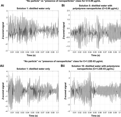
Figure 5 Single-sided amplitude spectrum of the Fast Fourier Transform (FFT) of filtered back-scattered signal portions of 60 seconds before being z-scored and acquired using distilled water and 100 nm nanoparticles solutions in concentrations of (A) 3.89 µg/mL and (B) 1.22E-03 µg/mL.
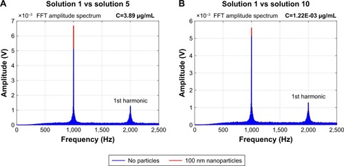
Table 3 Summary of the 53 features used in classes distinction
Figure 6 Scheme explaining the intuition behind the LDA, considering a two class problem (class A and class B) and a two-dimensional original features space (2D, composed of two features).
Notes: Original data samples are then projected to a lower features dimensional space, composed of a single feature (1D, one-dimensional, line). The separation line is calculated in order to maximize the “separability” of the projected samples. Abbreviation: LDA, Linear Discriminant Analysis.
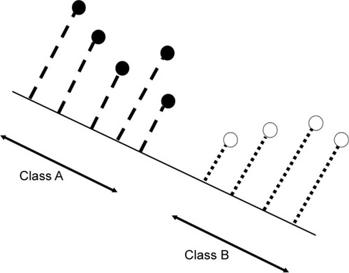
Figure 7 2D representation of the mean projected values considering each different acquisition spots and classes for the two final LDA features and corresponding separation line for nanoparticles concentration values (A) 55.38 µg/mL; (B) 37.59 µg/mL; (C) 19.14 µg/mL; (D) 3.89 µg/mL; (E) 0.16 µg/mL; (F) 1.56E-02 µg/mL; (G) 3.90E-03 µg/mL; (H) 2.44E-03 µg/mL; and (I) 1.22E-03 µg/mL. Red dots represent the class “no particles” and blue squares represent the class “presence of nanoparticles”.
Abbreviation: LDA, Linear Discriminant Analysis.
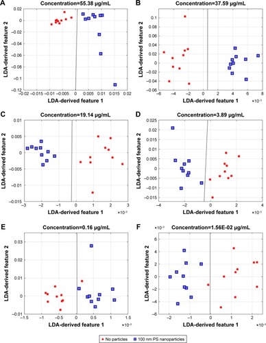
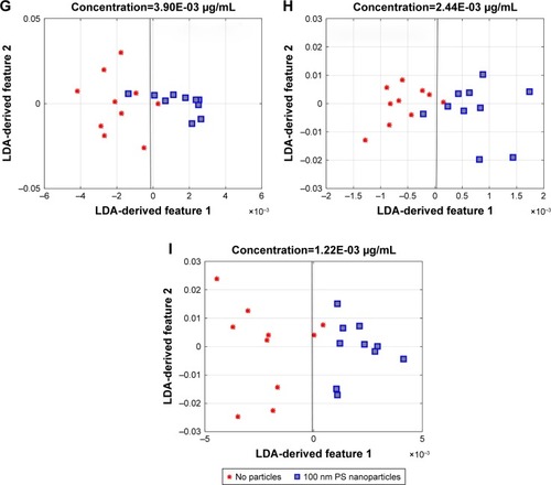
Figure 8 The five most important features for binary distinction problems involving nanoparticles solutions with concentrations of 1.22E-03 (solution 10), 2.40E-03 (solution 9), 3.90E-03 (solution 8), 1.56E-02 (solution 7), 0.16 (solution 6), 19.14 (solution 4), 37.59 (solution 3), and 55.38 µg/mL (solution 2), according to LDA and corresponding coefficients magnitude.
Abbreviation: LDA, Linear Discriminant Analysis.
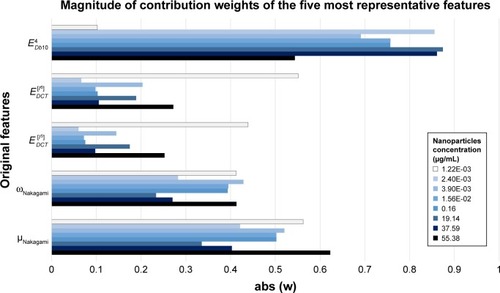
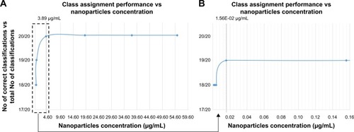
Figure 9 Number of correct class assignments (signal acquisition spots classified) vs total number of class assignments performed for (A) all nanoparticles concentration solutions; and (B) zoom in of (A) for low nanoparticles concentration values.