Electrospun Icariin-Loaded Core-Shell Collagen, Polycaprolactone, Hydroxyapatite Composite Scaffolds for the Repair of Rabbit Tibia Bone Defects

Figures & data

Scheme 1 Schematic illustration of the fabrication process of PCL/COL/HA/ICA composite scaffold.

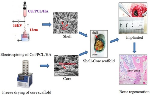
Figure 1 Surface topography and physical properties of the CPH scaffolds. (A1) The gross appearance of the uncross-linked scaffolds. (A2–A3) Scanning electron microscopy images of the uncross-linked scaffolds. (B1) The gross appearance of the cross-linked scaffolds. (B2–B3) Surface topography of the cross-linked scaffolds. (C) Water absorption ratios. (D)Porosity. (E) Loss weight; and mechanical property (F) of the scaffolds with and without cross-linking. (G) Spectra of the CPHI scaffolds with and without cross-linking. (H) Characterization of the hydroxyapatite (HA)-incorporated scaffolds. The results are presented as the mean ± standard deviations (n = 3). * p < 0.05; ** p < 0.01; * is the significance compared to the uncross-linked scaffolds.

Abbreviation: HA, hydroxyapatite.

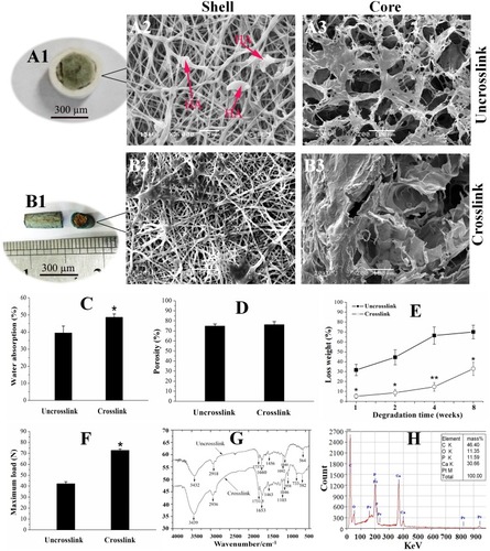
Figure 2 Characterization of microspheres, cumulative release of ICA and distribution. (A) Scanning electron microscopy images of the ICA loaded chitosan microspheres. (B) The curve of ICA released from the microspheres. (C) and (D) The scaffolds scanning electron microscopy images of the core scaffold, (C) without the chitosan microspheres, (D) with the chitosan microspheres. The results are presented as the mean ± standard deviations (n = 3). Red arrow: chitosan microspheres.

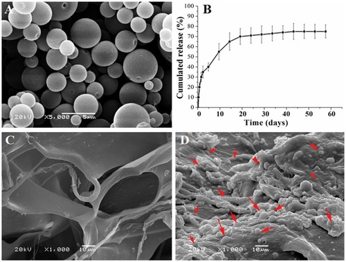
Figure 3 Adhesion and proliferation of rMSCs on the shell and core scaffolds. (A) Cell adhesion and proliferation on the shell scaffolds were demonstrated by SEM (A1 and A2), hematoxylin and eosin (H&E) staining (A3) and fluorescence staining (A4–A6). (B) Cell adhesion and proliferation on the core scaffolds were demonstrated by SEM (B1 and B2), H&E staining (B3) and fluorescence staining (B4–B6). Blue = DAPI staining for Nucleus. Red = scaffold (autofluorescence of genipin). Red arrows: cells. Scale bar = 100 µm.

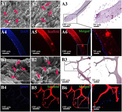
Figure 4 Implantation procedure, X-ray and 3D reconstruction analysis of new bone. (A) Photographs showing the surgical implantation procedure (A1 and A2) of the CPH, and CPHI scaffolds in rabbit bone defects. (A3) shows the defect control covered by the connective tissue after 12 weeks. (B1–B6) New bone formation of CPH and CPHI groups after 4, 8, and 12 weeks. (C1–C9) Evaluation of in vivo bone formation: representative X-ray images showing the level of the regenerated bone tissue after 4–12 weeks. (D1–D9) 3D reconstruction images showed the different reparative effects of the CPH and CPHI scaffolds after 4–12 weeks. Red arrows: bone density, Red dotted circles: defect areas, Red arrow: density bone regeneration.

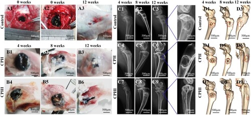
Figure 5 Micro-CT analysis of new bone. (A) Micro-CT scan images showing the level of regenerated bone tissue after 4–12 weeks. (B) Bone mineral density (BMD) of the regenerated bone tissue after 4–12 weeks. (C) Tissue connective density (Conn.Dn) of the regenerated bone tissue after 4–12 weeks. Data display the mean relative values calculated from three independent experiments (mean ± SD). * p < 0.05; ** p < 0.01; * is the significance compared to defect control, ^#is the significance compared to 8 weeks. Red dotted circles: defect areas.

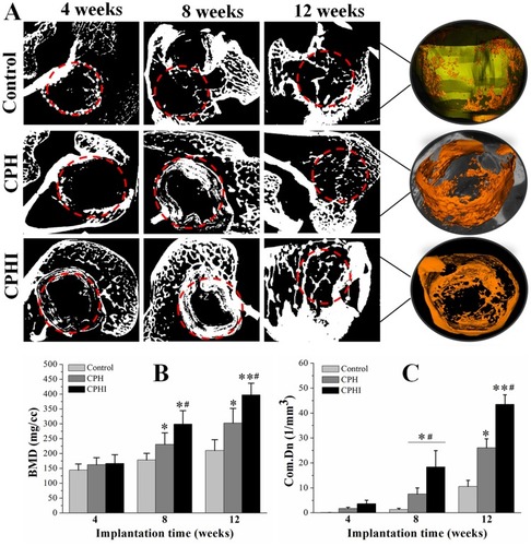
Figure 6 Histological staining assessment of the newly formed bone at 4–12 weeks post implantation of CPH and CPHI scaffolds in rabbit bone defects. (A) Staining with haematoxylin and eosin (H&E) demonstrates new bone formed in the CPH and CPHI scaffolds. (B) Masson’s trichrome shows matrix distribution (scale bar = 100 µm). (C) and (D) Show the quantitative data from (A) and (B), respectively. Data display the mean relative values calculated from three independent experiments (mean ± SD). * p < 0.05; ** p < 0.01; *** p < 0.001; * is the significance compared to defect control, ^# p < 0.05; is the significance compared to CPH group.

Abbreviations: NB, new bone; M, implanted material; HB, host bone; F, fibrous tissue.

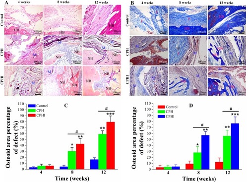
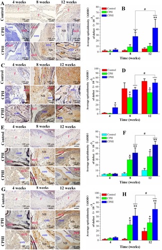
Figure 7 Immunohistochemistry staining for (A) alkaline phosphatase (ALP), (C) type I collagen (COL1), (E) osteocalcin (OC), and (G) osteopontin (OPN) of bone defects at 4–12 weeks post implantation in rabbits. (B), (D), (F), and (H) Show the quantitative data from (A), (C), (E), and (G), respectively. Data display the mean relative values calculated from three independent experiments (mean ± SD). * p < 0.05; ** p < 0.01; * is the significance compared to defect control, ^# p < 0.05; is the significance compared to CPH group. Scale bar = 100 µm.

Abbreviations: NB, new bone; F, fibrous tissue.