Figures & data
Figure 1 The characterization of MCM-41, SBA-15, and DMSN. (A, C and E) The representative SEM images and (B, D and F) TEM images of MCM-41, SBA-15, and DMSN. (G) The nitrogen adsorption−desorption isotherms and (H) the pore size distribution were measured according to the BET & BJH model. (I) The particle size and (J) zeta potential were measured.
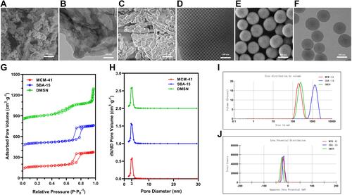
Figure 2 The potential pro-inflammation effects after various treatments within 7 days. (A) The body weight changes and the serum level of (B) TNF-α and (C) IL-1β were measured. (n=10, mean ± SD). (D–G) The histology examination of colon via H&E staining. Black arrow indicated the potential site of inflammation.
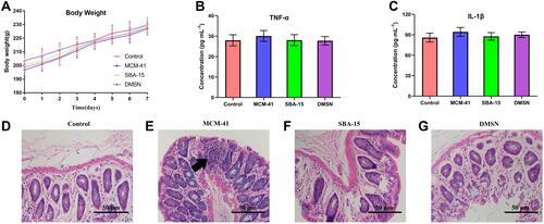
Figure 3 The diversity of gut microbiota. Results were shown as violin plot, the width of the shaded area represents the proportion of the data. (A) The Chao1 index; (B) ACE index; (C) The Shannon index; (D) Simpson index at day 3 and day 7. (n=10, mean ± SD).
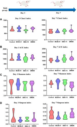
Figure 4 The differences of microbiota between groups. The Circos graphs at day 3 and day7, while the left semicircle represents the phyla composition of each group, and the right semicircle indicates the distribution of each phylum in the different groups. (n=10).
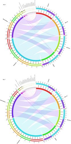
Figure 5 PCoA of the different treated groups at the OTU level at day 3 and day 7 (n=10).
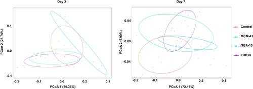
Figure 6 Specific taxa detection. Bacterial differences between (A) groups at day 7 were detected by LEfSe and (B) species with LDA score (log 10) >3.0 were plotted (n=10).
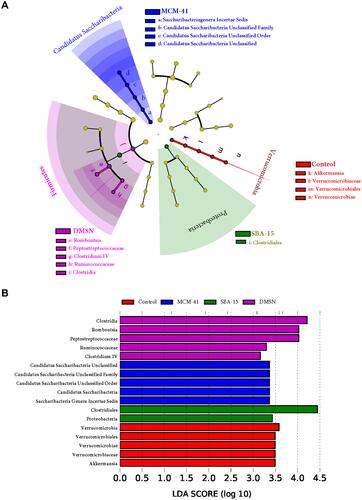
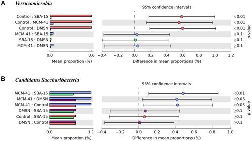
Figure 7 Multiple groups comparison at day 7. Specific phylum One-way ANOVA bar plot. (A) Verrucomicrobia: p value of Control and SBA-15<0.01, Control and MCM-41<0.01, Control and DMSN<0.01. (B) Candidatus Saccharibacteria: p value of MCM-41 and SBA-15<0.01, MCM-41 and DMSN<0.05, MCM-41 and Control<0.05.