pH-Responsive Nanoparticles for Enhanced Antitumor Activity by High-Intensity Focused Ultrasound Therapy Combined with Sonodynamic Therapy

Figures & data

Scheme 1 Schematic illustration of pH-responsive Ca@H NPs-mediated tumor theranostics including i) CO₂ generation, HMME release in the acidic tumor microenvironment, ii) CO₂/HMME-enhanced PA imaging, iii) CO₂ bubbles-enhanced HIFUT, and iv) HMME-mediated SDT for the residual lesions.

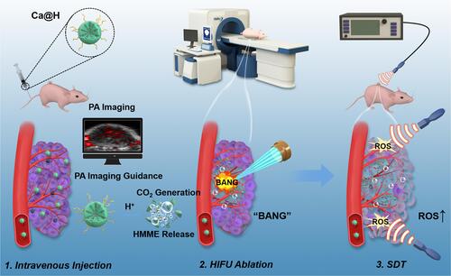
Figure 1 (A) Schematic illustration for fabrication of Ca@H NPs. (B) SEM and (C) TEM images of Ca@H. (D) Hydrodynamic diameter of Ca@H NPs detected by DLS. (E) Surface zeta potential of Ca@H NPs in aqueous solution. (F) UV-Vis spectra of free HMME, and Ca@H suspension.

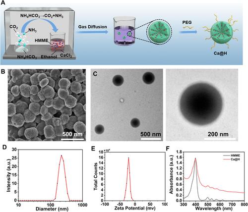
Figure 2 (A) Schematic diagram of the pH-activated Ca@H decomposition. (B1) Schematic illustration of the quantitative measurement of CO₂ using an air quality meter. (B2) CO₂ production diagram of different Ca@H concentrations in buffers at various pH. (C) Time-dependent size of Ca@H at different pH values (n = 3). (D) The relative released percentage of HMME from Ca@H under various pH (n = 3). (E) TEM images of Ca@H in acid buffer (pH = 6.5 or 5.5, stirring for 2 h). (F1) Schematic illustration of in vitro ROS generation upon US irradiation. (F2) ROS generation of Ca@H at different pH. (F3) Time-dependent ROS generation of Ca@H (pH = 5.5).

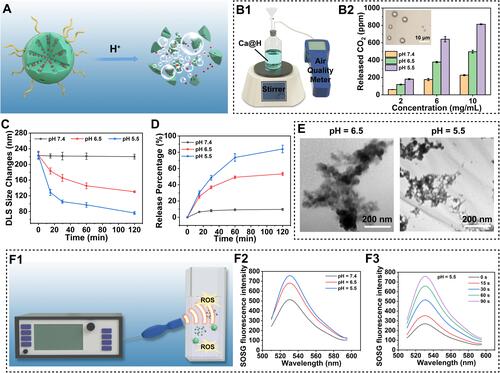
Figure 3 (A) CLSM images of 4T1 cells incubated with Ca@H in neutral or acid medium for 2 h and 4 h and (B) the correspond relative endocytosis rates of Ca@H analysed by flow cytometry. (C) CLSM images of intracellular ROS generation detected by DCFH-DA probe after various treatments. (D) Quantitative analysis of ROS generation in 4T1 cells after various treatments.

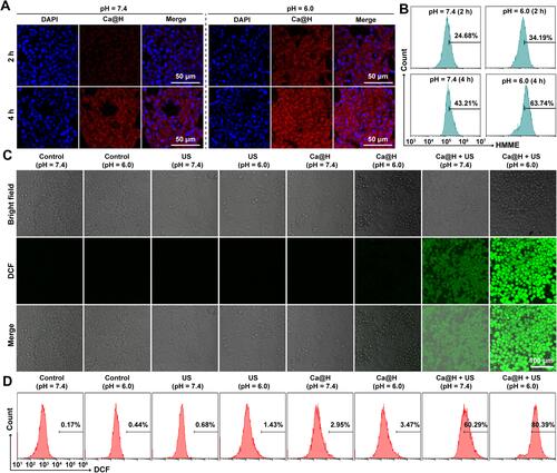
Figure 4 (A) Cytotoxicity of Ca@H after incubation with 4T1 cells at different concentrations of Ca@H for 4 h, 12 h and 24 h (n = 5). (B) Cell viabilities of 4T1 cells after various treatments (n = 5, t test, *p < 0.05, **p < 0.01, ***p < 0.001). (C) CLSM images of cells co-stained with CAM and PI after different treatments.

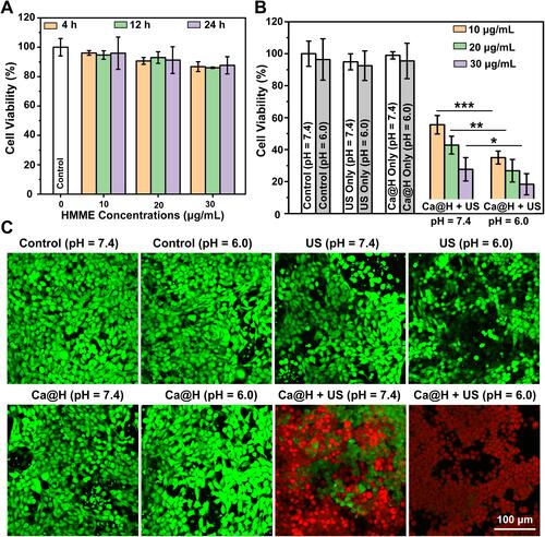
Figure 5 (A) Schematic illustration of the ex vivo HIFU ablation. (B) Representative US images of bovine liver tissues before and post HIFU ablation (the green circles indicate the areas focused by HIFU). (C) Gray scale value changes of bovine liver tissues after HIFU ablation (n = 3, t test, **p < 0.01). (D) The corresponding digital photos of bovine liver tissues after HIFU ablation. (E) Tissue volume changes of HIFU ablation (n = 3, t test, *p < 0.05). (F) H&E staining of bovine liver tissue after HIFU ablation (the red circles represent the damaged areas after HIFU irradiation).

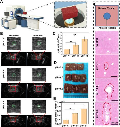
Figure 6 (A) In vitro PA images of CaCO₃ or Ca@H dispersed in buffers at various pH and (B) quantitative analysis of PA signal intensities (n = 3). (C) In vivo PA imaging at different time points. (D) In vivo PA signal increase (%) compared to pre-injection of Ca@H (n = 5, t test, ***p < 0.001).

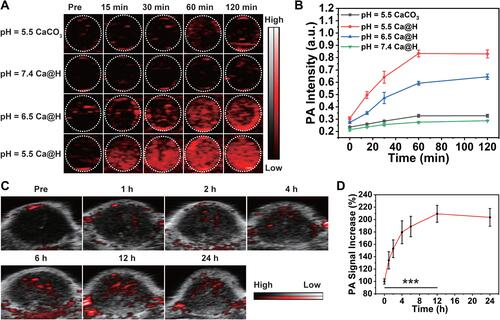
Figure 7 (A) Schematic illustration of the in vivo HIFU ablation. (B) Representative US images of tumor tissues before or post HIFUT with and without administration of Ca@H (the green circles indicate the areas focused by HIFU). (C) Gray scale value changes of tumor tissues after HIFU ablation with and without administration of Ca@H (n = 3, t test, **p < 0.01). (D) H&E staining of tumor tissues exposed to HIFU with and without administration of Ca@H (the red circles represent the damaged areas after HIFU irradiation).

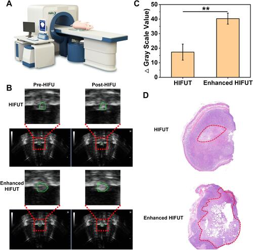
Figure 8 (A) Experimental design of the in vivo treatment. (B) Digital photos of 4T1 tumor bearing mice before and post various treatments. (C) Tumor growth curve of 4T1 tumor-bearing mice after various treatments (n = 5, t test, *p < 0.05). (D) Digital photo of tumors after various treatments. (E) Weight of tumor tissues excised from each group (n = 5, t test, *p < 0.05, **p < 0.01). (F) Tumor inhibition rates after different treatments (n = 5, t test, *p < 0.05, **p < 0.01). (G) Body weight of mice during the therapeutic period (n = 5).

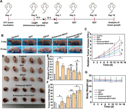
Figure 9 (A) H&E and PCNA staining of tumor tissues after various treatments. (B) H&E staining of major organs of mice after various treatments.

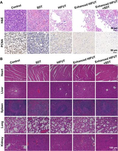
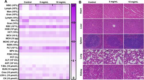
Figure 10 (A) Haematological analysis of mice after intravenously injected with Ca@H. (B) H&E staining of major organs excised from Ca@H treated-mice.