Development and in vivo Evaluation of Hydroxy-α-Sanshool Intranasal Liposomes as a Potential Remedial Treatment for Alzheimer’s Disease

Figures & data

Figure 1 HPLC analysis.

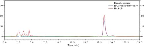
Table 1 Screening the Preparation of Hydroxy-α-Sanshool Nano-Liposomes

Treatment	HAS : Lipid Material (Mass Ratio)	Cholesterol : Soy Lecithin (Mass Ratio)	Ultrapure Water (mL)
1	1 : 15	1 : 3	15
2	1 : 20	1 : 4	15
3	1 : 25	1 : 5	15
4	1 : 25	1 : 4	20
5	1 : 20	1 : 3	20
6	1 : 15	1 : 5	20
7	1 : 15	1 : 4	25
8	1 : 20	1 : 3	25
9	1 : 25	1 : 5	25

Figure 2 Flowchart of animal experiment.

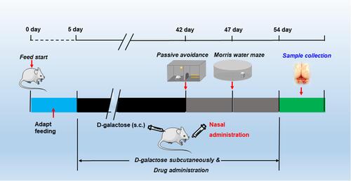
Table 2 Neuronal Injury Scoring Standard

Score	Diagnostic Criteria (Percentage of Damage)
0	0
0.5	< 10%
1.0	10% – 30%
1.5	30% – 50%
2.0	50% – 70%
2.5	70% – 90%
3.0	> 90%

Table 3 Encapsulation Efficiency and Loading Capacity of HAS-LPs in Each Formulation

No	Encapsulation Efficiency (%)	Loading Capacity (%)	Particle Size (nm)	PDI	Zeta Potential (mV)
1	48.24 ± 3.76	3.02 ± 0.13	210.29 ± 12.76	0.332 ± 0.097	−28.9 ± 5.77
2	73.19 ± 3.51	4.07 ± 0.20	181.77 ± 2.73	0.207 ± 0.038	−53.8 ± 2.78
3	55.72 ± 2.14	2.14 ± 0.07	208.41 ± 7.64	0.326 ± 0.076	−28.7 ± 5.65
4	52.68 ± 2.63	2.03 ± 0.12	196.86 ± 5.06	0.269 ± 0.064	−39.9 ± 5.69
5	56.12 ± 1.47	2.67 ± 0.16	191.05 ± 5.58	0.235 ± 0.078	−36.1 ± 4.99
6	63.67 ± 2.18	3.98 ± 0.21	188.09 ± 3.65	0.223 ± 0.052	−49.6 ± 3.63
7	59.85 ± 2.63	3.74 ± 0.20	190.73 ± 4.89	0.231 ± 0.066	−46.2 ± 3.25
8	57.87 ± 1.95	2.76 ± 0.18	203.69 ± 6.38	0.296 ± 0.056	−31.3 ± 5.24
9	54.29 ± 1.29	2.09 ± 0.15	199.32 ± 5.12	0.278 ± 0.072	−42.5 ± 5.62

Figure 3 (A) Schematic illustrating the process used to prepare hydroxy-α-sanshool nanoliposomes. (B) Morphology of HAS-LPs. (C) Size distribution of HAS-LPs after storage for 0, 1 (25 °C) and 8 (4 °C) weeks. (D) Zeta potential of HAS-LPs after 0, 1 (25 °C) and 8 (4 °C) weeks. (E) HAS contents in free HAS and HAS-LPs after storage at 25 °C for 1 week and 4 °C for 8 weeks.

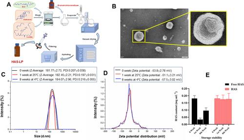
Figure 4 (A) Schematic illustration of the determination of hydroxy-α-sanshool nano-liposomes release. (B) The continuous Release curve of HAS and HAS-LP in vitro. (C) Release model of the group of HAS. (D) Release model of the group of HAS-LP.

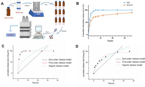
Figure 5 HE staining of nasal mucosa (the green arrow showed congestion of blood vessel, yellow arrow showed lamina propria necrosis, green arrow showed epithelial cell necrosis and blue arrow showed inflammatory cell infiltration).

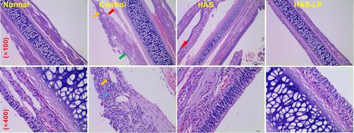
Figure 6 HAS-LP treatment attenuated learning and memory deficits in the passive avoidance test. (A) The escape latency. (B) The number of errors. Data are expressed as means ± S.D. (n = 8). **P < 0.01 vs the control group; *P < 0.05 vs the control group.

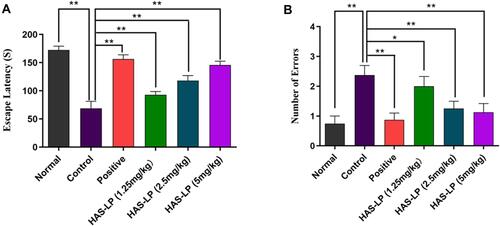
Figure 7 HAS-LP treatment attenuated learning and memory deficits in the Morris water maze test. (A) The mean escape latency time in the training trials. (B) The number of crossing platforms. (C) The residence time spent in the target quadrant. Data are expressed as means ± S.D. (n = 8). **P < 0.01 vs the control group.

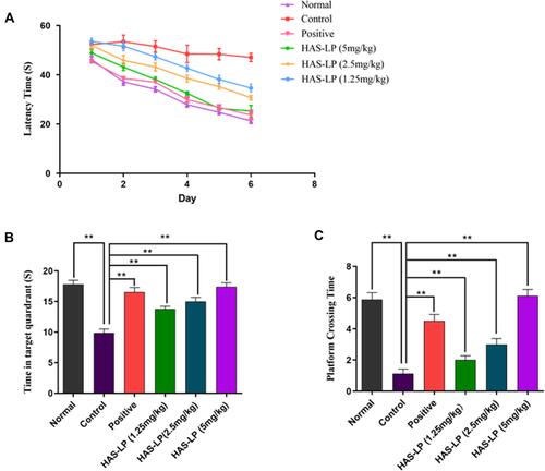
Figure 8 HAS-LP treatment attenuated hippocampal neuronal damage and loss. (A) Representative photomicrographs of HE staining and Nissl staining in the hippocampal CA1 and CA3 regions are shown (magnification, 40× and 400×). (B) The damage index of D-galactose model mice (mean ± SD, n = 5) and the number of Nissl bodies of D-galactose model mice (mean ± SD, n = 5). *P < 0.01, **P < 0.05 vs the control group.

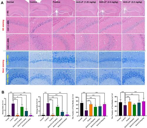
Figure 9 Continued.

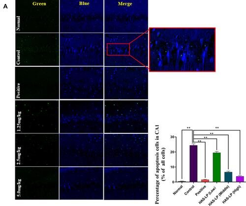
Figure 9 (A) Representative photomicrographs of Tunel staining in the hippocampal CA1 regions (magnification, 400×) and the percentage of apoptotic cells in the CA1 region of D-galactose model mice (mean ± SD, n = 5) are shown. (B) Representative photomicrographs of Tunel staining in the hippocampal CA3 regions and the percentage of apoptotic cells in the CA3 region of D-galactose model mice (mean ± SD, n = 5) are shown (magnification, 400×). **P < 0.05 vs the control group.

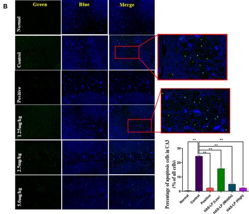
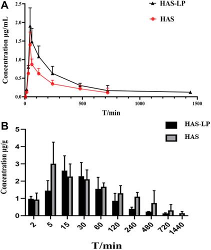
Table 4 Pharmacokinetic Parameters of Free HAS and HAS-LP in Plasma and Brain Tissue (n=5, Mean ± SD) **P < 0.01 vs HAS Group; *P < 0.05 vs HAS Group

Pharmacokinetic Prameters	Plasma		Brain Tissue
	HAS	HAS-LP	HAS	HAS-LP
AUC0-t (mg h^−1 L^−1)	5.111±1.199	8.795±1.428**	7.438±1.735	15.787±2.854**
MRT0-t (h)	4.178±0.565	6.296±1.022**	3.074±0.618	6.412±1.481**
t1/2 (h)	4.140±0.893	4.444±0.754	5.116±0.729	6.734±1.011*
tmax (h)	0.500±0.194	0.500±0.052	0.250±0.059	0.083±0.030
Cl (L h^−1 kg^−1)	0.842±0.178	0.56±0.206*	None	None
Cmax (mg L^−1)	1.398±0.289	1.906±0.343**	2.613±0.457	3.015±1.305*

Figure 10 (A) Time profile of the plasma HAS level of mice after they were nasally administered with free HAS and HAS-LP. (B) Time profile of the brain tissue HAS level of mice after they were nasally administered with free HAS and HAS-LP.