Figures & data
Figure 1 Particle size distribution of the three magnetic tracers by dynamic light scattering.
Note: The particle size (logarithmic scale) is shown against the intensity.
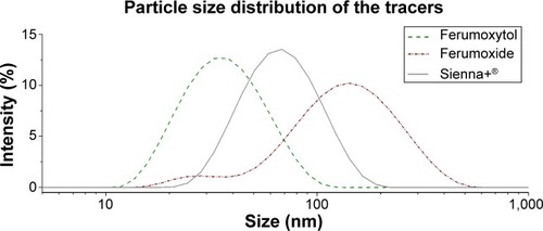
Figure 2 Relationship between the time after injection of the magnetic tracer and successful identification of transcutaneous hotspot.
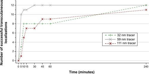
Figure 3 Boxplots of the relationship between the magnetic tracer and: (A) the number of excised sentinel lymph nodes during surgery; (B) the ex vivo magnetometer counts of the excised sentinel lymph nodes; (C) the iron content measured of the excised sentinel lymph nodes by vibrating sample magnetometry.
Notes: The circle symbols represent outliers; the diamond symbols represent the mean value.
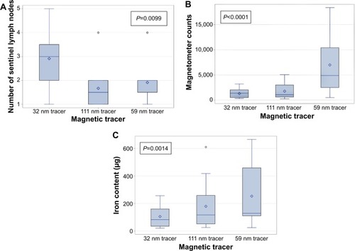
Figure 4 Correlation between the iron content as determined by vibrating sample magnetometry and the ex vivo magnetometer counts for the different magnetic tracers.
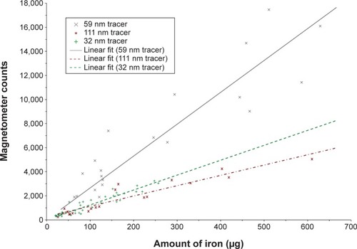
Figure 5 Iron distribution within nodes on histopathology using Perl’s Prussian blue staining for iron and haematoxyline & eosine.
Notes: Magnification 2×, with inserts at 20× magnification. (A) Node containing the 111-nm tracer; (B) node containing the 59 nm tracer; (C) node containing the 32 nm tracer.
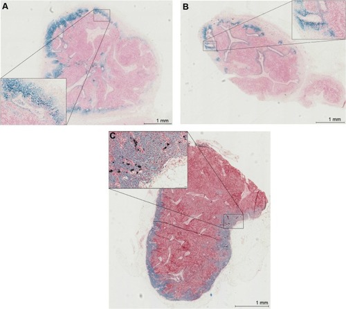
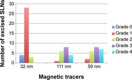
Figure 6 Number of excised sentinel lymph nodes (SLNs) per grade of iron distribution, for the three different magnetic tracers.
Note: Grade 0 = none, Grade 1 = minimal, Grade 2 = mild, Grade 3 = moderate, and Grade 4 = marked.