Prognosis and Personalized Treatment Prediction in Different Mutation-Signature Hepatocellular Carcinoma

Figures & data

Figure 1 The flow gram of this study.

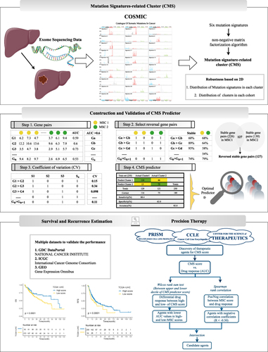
Figure 2 Mutation signature landscape in HCC and the clinical applications of a mutation-signature related cluster. (A) Waterfall plot of top 30 genes with significantly mutation of HCC patients. (B) Six mutation signatures extracted using NMF in HCC. (C) NMF identifies two clusters of LIHC patients with distinct mutation signatures. (D) Cophenetic curve for a different number of clusters. (E) Pie charts indicate the fraction of distinct mutation signatures in all samples, MSC1, and MSC2 HCC patients. (F and G) Kaplan–Meier curve of overall survival (F) and relapse-free survival (G). (H and I) Univariant Cox regression for overall survival (H) and relapse-free survival (I). (J and K) Multivariant Cox regression for overall survival (J) and Relapse free survival (K). (L) Cox regression analysis stratified by stage and vascular invasion.

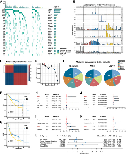
Figure 3 The development of a robust classification predictor depends on four steps. Step 1. Datasets with prognostic information were retrieved and processed, and 634 genes with AUC >0.6 between tumor and normal samples were selected. Step 2. Construction of gene pairs, identification of 130 stable reversed gene pairs, and further selection relying on LASSO regression model. Step 3. Construction and validation of the LASSO logistic model in the train and test cohorts. Step 4. Prognosis prediction in five cohorts with prognosis information (GSE14520, GSE76427, GSE114269, GSE54236, ICGC).

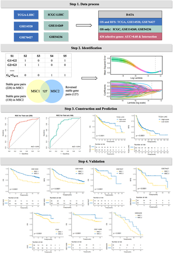
Figure 4 Underlying biologic function and distinct immune microenvironment patterns of two CMSs. (A–C) Gene set enrichment analysis (GSEA) of GO (A), KEGG (B), and cancer hallmark gene sets (C) according to the MSCs. (D) Immune cell infiltration calculated by CIBERSORT algorithm. (E) The expression of specific co-inhibitory and co-stimulatory immune checkpoints (ICPs) in two clusters. (F) immune indicators were collected and compared between two CMSs. (G and H) The TIDE algorithm was used to predict the immune status including exclusion and dysfunction and estimated the sensitivity (G) of two MSCs to immunotherapy (H) in the TCGA cohort. (I) SubMap analysis manifested that the MSC1 could be more sensitive to the anti-PD-1 therapy. *P <0.05, **P <0.01.

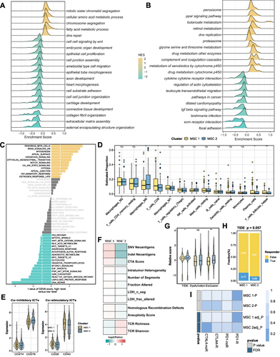
Figure 5 The multi-omics landscape of the MSCs. (A) Mutation landscape (right) and frequency (left) of the top 30 FMGs in TWO MSCs. (B and C) Differences in TMB (B) and neoantigen (C) between two CMSs. (D) The relation dot plot for TMB and predictor score. (E) CNV landscape (right) and frequency (left) of top 30 FHGs in two MSCs. (F–H) Differences of arm gain (F), focal gain (G), FGG (H) between two groups. (I and J) Differences of methylation drive genes in methylation level (I) and mRNA expression level (J). *P <0.05, **P <0.01, ***P <0.001.

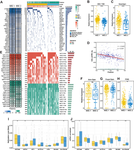
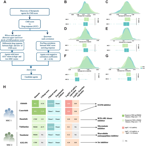
Figure 6 Identification of candidate agents with higher sensitivity in MSC1, high-risk patients. (A) Schematic outlining the strategy to identify agents with higher drug sensitivity for MSC1 patients. (B–G) Identification of six potential therapeutic agents using estimated AUC. (H) Identification of most promising therapeutic agents for two MSCs according to the evidence from multiple sources, including CMap dataset, experimental and clinical evidence, as well as expression at both the mRNA and protein levels.