Figures & data
Figure 1 Measurement setup for the nasal sound pressure method. The amplitude-modulated driver stage, including the Agilent 35670A, the Agilent 33220A, and the transmitter inductive link, is driving the implant. The nasal sound pressure is measured by a microphone with a pre-amplifier and is analyzed by the Agilent 35670A.
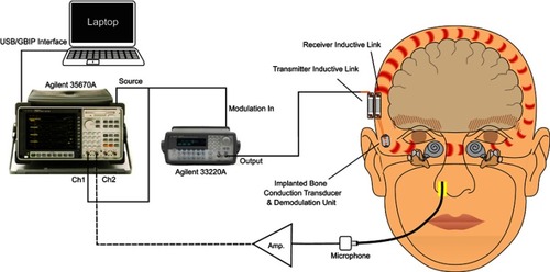
Figure 2 The nasal sound pressure for patient 12 at surgery, fitting, and follow-up visits at 1, 3, 6, and 12 months after fitting. The noise floor from surgery is also presented.
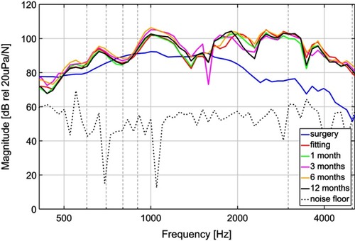
Figure 3 Average nasal sound pressure level based on follow-up data for each patient (in colors) together with the overall mean (black solid line) and the average noise floor (black dotted line).
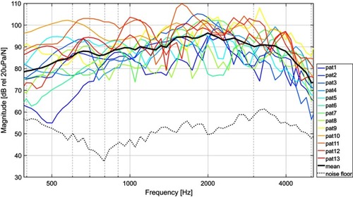
Figure 4 Boxplot of the nasal sound pressure of all patients at surgery at frequencies 0.5, 1.0, 2.0, and 4.0 kHz, showing average (*), median (red line), 25 and 75 percentiles (blue box), and minimum and maximum values (whiskers).
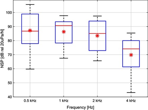
Figure 5 Linear model of the nasal sound pressure over time relative to baseline (fitting) at four frequencies with the respective equation showing slope and intercept.
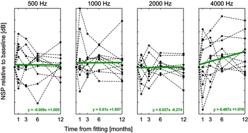
Figure 6 Random effects visualization: for each patient included in the analysis, the individual k-value is estimated with its 95% CI. Intervals not including 0 indicate that the patient has a significant deviation from the overall slope (group average), marked with a red asterisk.
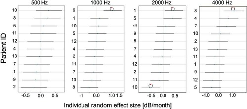
Table 1 Summary of results from model fitting. For the selected frequencies, a summary of the estimated fixed effects with their standard error for the linear mixed effects model is given. t-values >2.0057 indicate a significant deviation from 0 (α=5%)
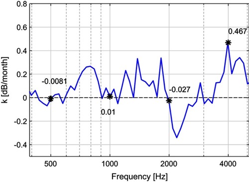
Figure 7 Slope value (k) as a function of frequency. Asterisks (*) mark the values at the audiometric frequencies.