
Figures & data
Figure 1 Milling process in otological surgery.
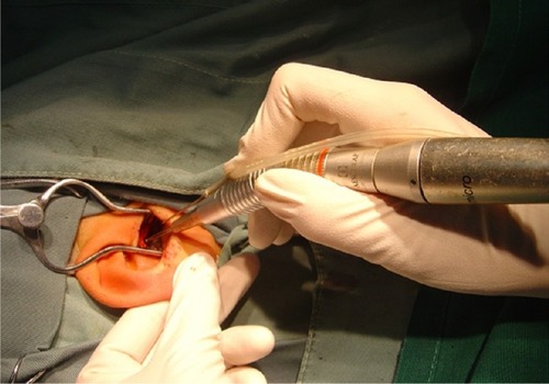
Figure 2 Force sensors on the sleeve.
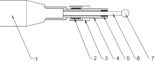
Figure 3 Modified drill system.
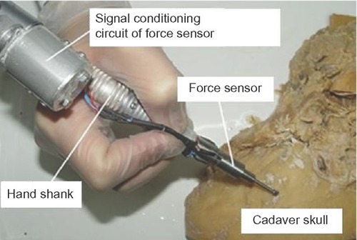
Figure 4 Collation map of the initial and reversed force signal of Fx and Fy.
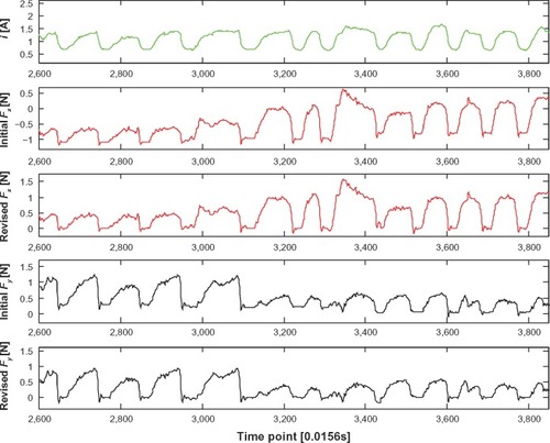
Figure 5 Current signal after starting the drill, when we find a slow decline in the current.
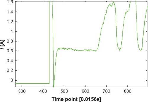
Figure 6 Scatter diagram of Fj and i during normal drilling and their fitting curve.
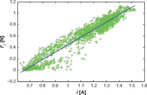
Figure 7 Comparison of i, Fj and kt during normal milling.
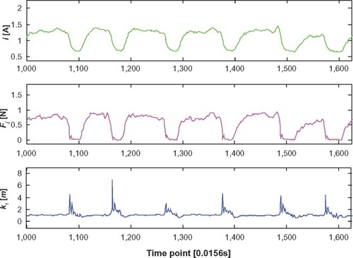
Figure 8 Functional relationship between f(m) and m, where the horizontal ordinate represents m and the vertical ordinate represents f(m).
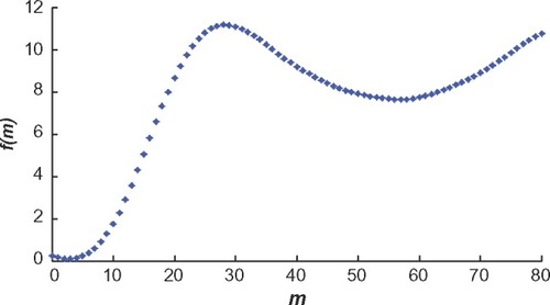
Figure 9 Comparison of the curve of kt when the m values are 0 and 2, where the horizontal ordinates represent time points and the vertical ordinates represent kt.
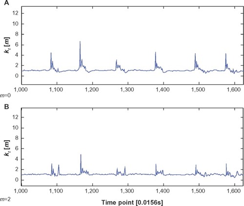
Figure 10 Curve graph between f(m) and m for m values of 2 to 3, where the horizontal ordinate represents m and the vertical ordinate represents f(m).
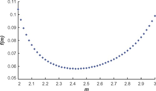
Figure 11 Comparison of the curve of kt for m values of 2 and 2.42.
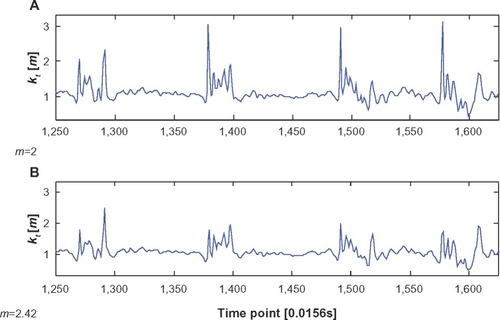
Figure 12 Sketch of the drill bit when it is milling through the bone wall.
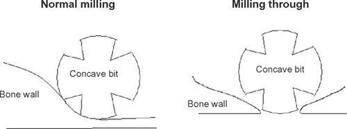
Figure 13 Recognition of milling through bone tissue wall.
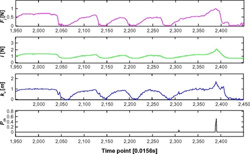
Figure 14 Recognition of entanglement with cotton swabs (the data in this figure was collected in the process of entanglement).
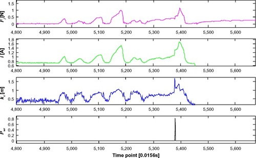
Table 1 Final results of the recognition method for abnormal milling states