Three-dimensional needle-tip localization by electric field potential and camera hybridization for needle electromyography exam robotic simulator

Figures & data

Figure 1 Overview of the robotic stimulator.

Notes: Image processing and electro-localization by phantom are used to estimate the 3D needle-tip location. According to the position of the needle and presumed pathological conditions, EMG waveform could be presented to the trainees.
Abbreviations: 3D, three dimensional; EMG, electromyography.

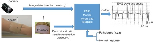
Table 1 Composition of muscle-equivalent phantom for 100×100×10 mm³ dimension

Materials	Amount (g)	Effect
Deionized water	100	Base material
Agar	3	Forming
Sodium dehydroacetate	0.05	Antisepsis
Sodium chloride	0.2	Conductivity

Figure 2 Experimental setup to evaluate the electric field potential and camera hybridization method to localize the needle tip: robotic hand, camera, and phantom.

Note: Purpose-built device is used to locate the needle at the desired position.

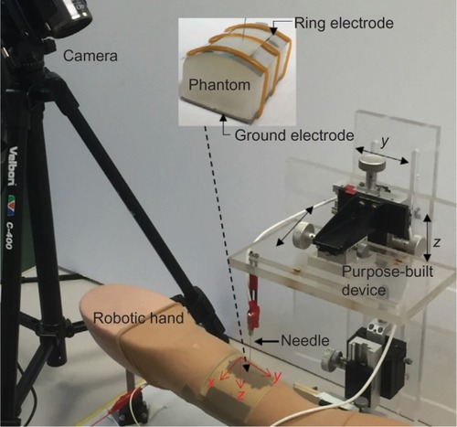
Figure 3 Needle localization method by electric field potential and camera hybridization.

Notes: (A) Measurement method of the voltage distribution, (B) segmentation steps to extract the needle. Images Ba and Bb are shown with a different contrast than the original for easier visualization. In image Be needle tip camera position localization method is shown, points A, B, C, and D describe the contour of measured area, points A', B', P and P' describe needle insertion point position information. Image Bc is the subtraction between images Ba and Bb. A gray filter is applied to segment needle in image Bd.

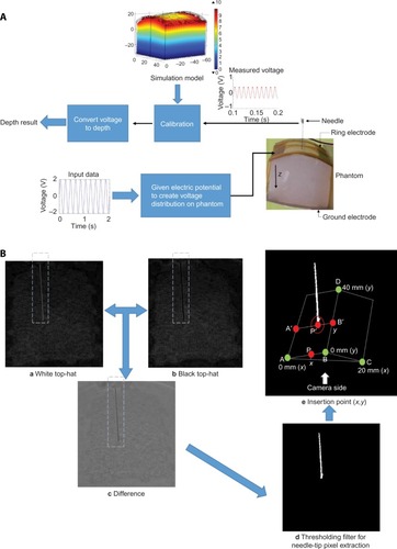
Figure 4 Calibration curves used to improve the estimation of needle penetration distance.

Notes: No calibration corresponds to a phantom with linear voltage distribution. Calibration curves are calculated using a simulation model of the phantom. Calibration 1 is generic for all insertion points and calibration 2 is specific for each insertion point (a measurement at x =5 and y =20 is shown as example).

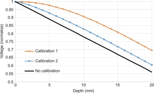
Figure 5 Measurement locations where needle is inserted to estimate the accuracy of the needle-tip localization.

Note: The interval of the measurement points for both x-axis and y-axis is 5 mm. Dots are the center region and triangles the border region on measured area.

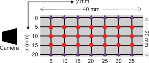
Figure 6 Average needle-penetration distance (z) from the voltage distribution of the phantom before and after voltage calibration: (A) All measurement results and (B) measurement in center region.

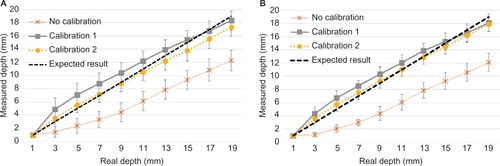
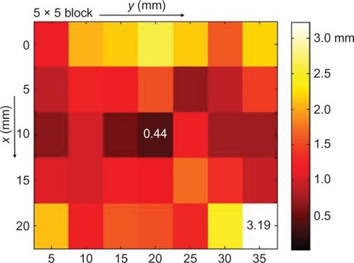
Figure 7 Image processing error (x,y) using 35 insertion points.

Note: Scale bar means the prediction error in mm.

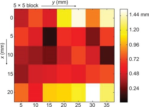
Figure 8 Needle-tip position error (x,y,z) along z-axis using electric field potential and camera hybridization.

Notes: Average and standard deviation are presented from 1 to 19 mm of depth. Solid line represents all measurements and dotted line shows the results of the center area.

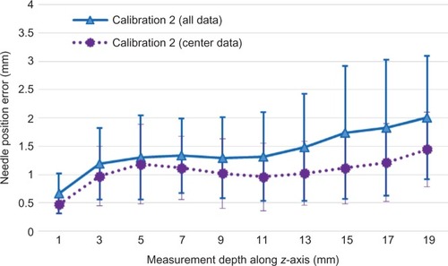
Figure 9 Needle-tip position error (x,y,z) seen from the surface using electric field potential and camera hybridization.

Note: Scale bar is the average of the error of all depths (1–19 mm).