
Figures & data
Figure 1 Result of automatic segmentation using fractal dimension on occipital area electrode signal from a patient with Jeavons syndrome.
Abbreviations: EEG, electroencephalography; FDFV, fractal dimension feature vector.
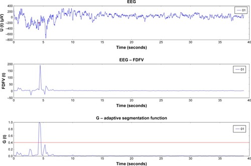
Figure 2 Schematic flow chart for set extraction and further processing (compression, classification using GP+SVM).
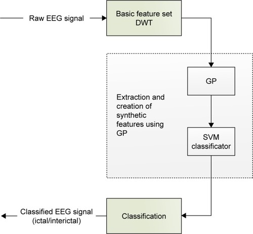
Figure 3 Population tree of suggested algorithm with two F functions (nodes) that make up new flagged vectors that are expressed by the offspring.
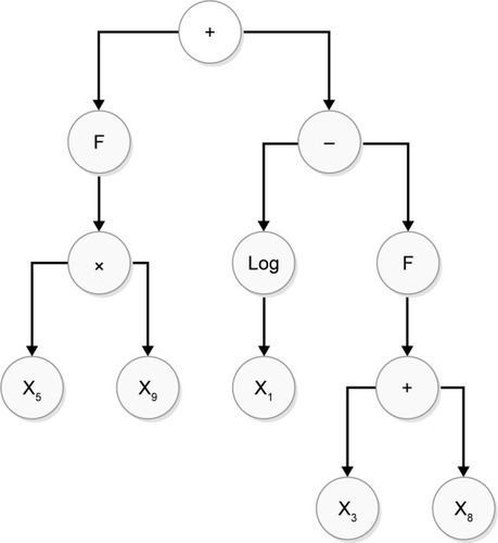
Figure 4 GP–SVM block scheme.
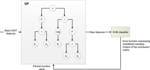
Table 1 Clinically diagnosed epilepsy types of patients
Table 2 Frequency bands for four-level DWT decomposition
Figure 5 Four-level DWT decomposition for interictal EEG.
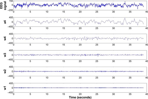
Figure 6 Four-level DWT decomposition for ictal EEG.
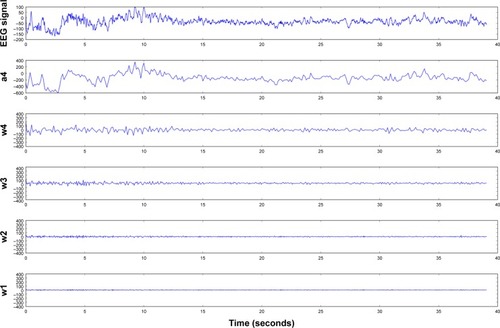
Table 3 Basic set feature vector mapping
Figure 7 Training stage of population tree samples separation. Population tree descendants combining the input features x9+x10 are clearly distinguishable from the population member genetically combining the input features x17+x18.
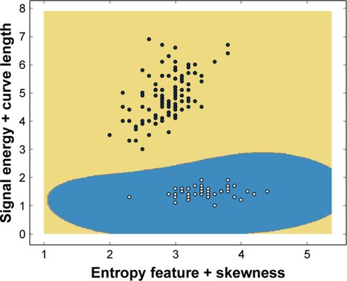
Figure 8 Confusion matrix for dataset shown in .
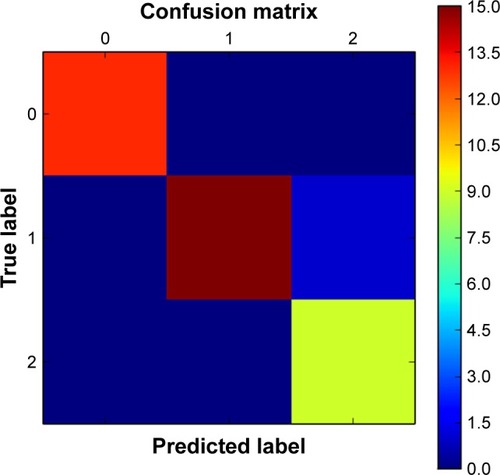
Table 4 Classification accuracy
Table 5 Compressed feature vector with compression level 5
Table 6 Compressed and basic feature vectors-based classification performance comparison