Figures & data
Figure 1 Experimental design. Experimental design and timeline of the two experimental sessions (Active and Sham).
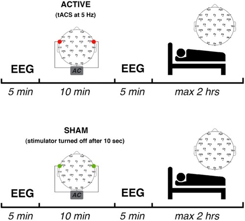
Table 1 Means And Standard Deviations (S.D.) Of Polysomnographic Variables In The Two Experimental Conditions
Figure 2 Effects of θ-tACS on sleep EEG activity. Topographic maps of the mean EEG power spectra (log-transformed) during the first NREM sleep cycle of the naps following the Active (θ-tACS, first column) and Sham (second column) stimulation and statistical maps of comparisons assessed by paired t-tests (θ-tACS vs sham, third column). Maps are plotted for the following frequency bands: slow-wave activity (SWA, 0.50–4.75 Hz), theta (5.00–7.75 Hz), alpha (8.00–11.75 Hz), sigma (12.00–15.75 Hz), and beta (16.00–24.75 Hz). Values are colour coded and plotted at the corresponding position on the planar projection of the scalp surface and are interpolated (biharmonic spline) between electrodes. The topographic maps (first and second columns) are scaled between minimal and maximal values of the spectral power considering the two experimental conditions within each frequency band. The minimum (blue number) and the maximum (red number) for each scale are also reported close to the corresponding maps. The statistical maps are scaled symmetrically according to the absolute maximal t-value across the statistical comparisons in all frequency bands.
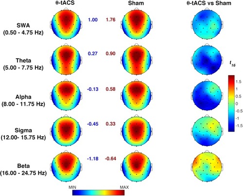
Figure 3 Time-course of EEG activity during the first NREM sleep cycle after sham and θ-tACS. The time-course of the spectral power in each frequency band during the first NREM sleep cycle of the naps following the Active (red line) and the Sham (blue line) for Fz, Cz, Pz, Oz representative cortical sites. The values were obtained by dividing the individual time period from the sleep onset to the first REM sleep (or the final awakening in absence of REM sleep) into 20 equal intervals and calculating the spectral power at each scalp location for each interval. Data were calculated for each subject, then averaged across subjects and the log-transformed values were plotted at the corresponding position on the planar projection of the scalp surface.
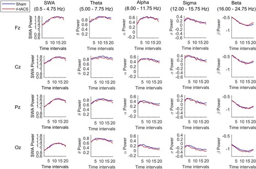
Table 2 Means And Standard Deviations (S.D.) Of Polysomnographic Variables In The Two Experimental Conditions For Responders And Non-Responders Groups
Figure 4 Effects of θ-tACS on sleep slow-wave activity (SWA) in responders. (A) Topographic distribution of the SWA power during the first NREM sleep cycle for Active (left) and Sham (central) conditions in responders to θ-tACS stimulation during wakefulness (n=7). The statistical map of the comparisons between the two experimental conditions by paired t-test is reported (right). Values are color coded, plotted at the corresponding position on the planar projection of the hemispheric scalp model and interpolated between electrodes. (B) Individual SWA power at C4 scalp location for Sham and Active conditions in responders.
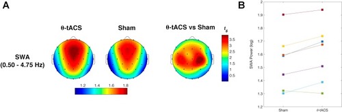
Figure 5 Time-course of slow-wave activity during the first sleep cycle in responders to θ-tACS. (A) The time-course of the spectral power for slow-wave activity (0.50–4.75 Hz) during the first NREM sleep cycle of the naps following the Active (red line) and the Sham (blue line) stimulations in the responders' subgroup. The values were obtained by dividing the individual time period from the sleep onset to the first REM sleep (or the final awakening in absence of REM sleep) into 20 equal intervals and calculating the spectral power at each scalp location for each interval. Data were calculated for each subject, then averaged across subjects and the log-transformed values were plotted at the corresponding position on the planar projection of the scalp surface. (B) Mean percentage difference in SWA power between Active and Sham condition for the time intervals of the first NREM sleep cycle. Positive values indicate the prevalence of SWA in Active relative to the Sham condition. Error bars show the standard error. (C) Responders’ topographic distribution of the rise rate of SWA (0.50–4.75 Hz) during the first NREM sleep cycle modelled by a linear least-squares regression on individual time-course data, separately for the two conditions. The statistical map of the comparisons between the two experimental conditions by the Wilcoxon test is reported. Values are color coded, plotted at the corresponding position on the planar projection of the hemispheric scalp model and interpolated between electrodes.
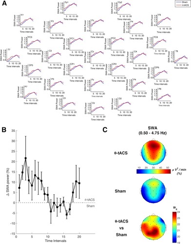
Figure 6 Relationship between θ-tACS EEG effects during wakefulness and SWA modulation in the subsequent sleep. Topographic distribution of the Spearman’s Rho coefficients (left) and corresponding p-values (right) of the correlations between the θ-tACS effect on theta EEG activity [percentage of theta power increase (post-/pre-stimulation) in the Active relative to Sham condition] and the effect on the SWA during the subsequent sleep (Active/Sham) computed on the whole sample. Values are colour coded, plotted at the corresponding position on the planar projection of the hemispheric scalp model and interpolated between electrodes.
![Figure 6 Relationship between θ-tACS EEG effects during wakefulness and SWA modulation in the subsequent sleep. Topographic distribution of the Spearman’s Rho coefficients (left) and corresponding p-values (right) of the correlations between the θ-tACS effect on theta EEG activity [percentage of theta power increase (post-/pre-stimulation) in the Active relative to Sham condition] and the effect on the SWA during the subsequent sleep (Active/Sham) computed on the whole sample. Values are colour coded, plotted at the corresponding position on the planar projection of the hemispheric scalp model and interpolated between electrodes.](/cms/asset/79fd1fe0-ead2-4657-a809-74a75004288f/dnss_a_12173978_f0006_c.jpg)
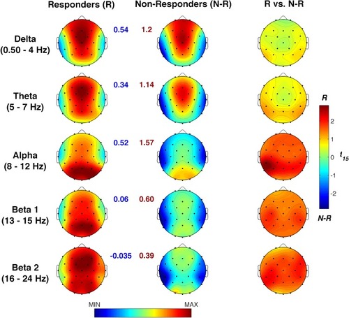
Figure 7 Baseline EEG differences during resting wake between responders and non-responders. Baseline topographic distribution of the waking EEG spectral powers in responders and non-responders and statistical maps of their comparisons by un-paired t-tests. Maps are plotted for the following frequency bands: slow-wave activity (SWA, 0.50–4.75 Hz), theta (5.00–7.75 Hz), alpha (8.00–11.75 Hz), sigma (12.00–15.75 Hz), and beta (16.00–24.75 Hz). Values are colour coded and plotted at the corresponding position on the planar projection of the scalp surface and are interpolated (biharmonic spline) between electrodes. The topographic maps (first and second columns) are scaled between minimal and maximal values considering the two experimental conditions within each frequency band. The minimum (blue number) and the maximum (red number) for each scale are also reported close to the corresponding maps. The statistical maps are scaled symmetrically according to the absolute maximal t-value across the statistical comparisons in all frequency bands.