An automated sleep-state classification algorithm for quantifying sleep timing and sleep-dependent dynamics of electroencephalographic and cerebral metabolic parameters

Figures & data

Figure 1 Comparison of human scoring to machine scoring.

Notes: Principal component plots of a 43-hour recording scored in 10-second epochs by a human (A) and using the machine learning algorithm (B). Each dot represents one 10-second epoch, and its color represents sleep state (SWS = blue, wake = red, REMS = orange). The computer-scored plot used data from 10 am to 2 pm (Zeitgeber time 4–8 in the first complete light/dark cycle of the recording) as training data to score every epoch in the entire 43-hour recording. Both for BALB/CJ mice (C) and C57BL/6J mice (D), the agreement between machine-scored and human-scored increased as more of the training data were used. For each genetic strain, 8,640 2-second epochs and 8,640 10-second epochs were scored by a human and by the autoscoring procedure, with 0.05%, 0.1%, 0.5%, 1%, 10%, 50%, 80%, and 100% of those 8,640 epochs used as training data. These correspond to 4 epochs, 9 epochs, 43 epochs, 86 epochs, 864 epochs, 4,320 epochs, 6,912 epochs, and 8,640 epochs, respectively. In each case it was ensured that at least one epoch of each state was present. Two measures of agreement between the human scoring and the machine scoring were computed: Cohen’s kappa and global agreement. The x-axis shows the percentage of the 8,640 epochs used as training data, indicating that the learning algorithm requires only about 1% of the training data to reach optimal performance.
Abbreviations: REMS, rapid-eye-movement sleep; SWS, slow-wave sleep.

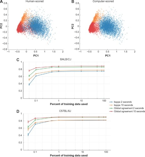
Figure 2 EEG and EMG data for comparison of human scoring and machine scoring.

Notes: The top two traces show human and autoscored sleep states for each 10-second epoch of the EEG and EMG shown in the lower panels. The sleep states are labeled with color (gray for wake, white for SWS, and black for REMS).
Abbreviations: EEG, electroencephalography; EMG, electromyography; REMS, rapid-eye-movement sleep; SWS, slow-wave sleep.

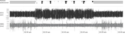
Figure 3 Agreement statistics between human scoring and machine scoring.

Notes: For the data scored in 10-second epochs, the agreement statistics compare the human and machine scoring for the entire 40–48-hour recording. For the data in 2-second epochs, the comparison is between 8,640 epochs that were scored by hand and the same 8,640 epochs scored by the automated scoring algorithm. Lines inside boxes represent median values. The lower end of each box indicates the first quartile of the data (Q1), and the upper end represents the third quartile (Q3). To draw the whiskers, we calculated the interquartile range (IQR), which is the distance between Q1 and Q3. The lower whisker indicates the lowest data point within 1.5 IQR of Q1. The upper whisker indicates the largest data point within 1.5 IQR of Q3. Outliers more than 1.5 IQR but less than 3 IQR above Q3 or below Q1 are represented with open circles.
Abbreviations: B6, C57BL/6J mice; BA, BALB/CJ mice; REMS, rapid-eye-movement sleep; SWS, slow-wave sleep.

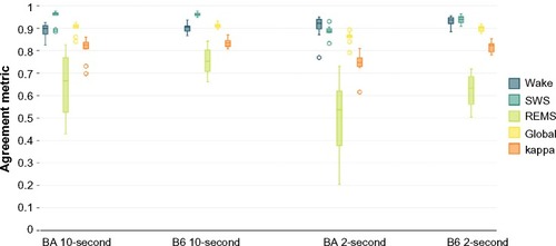
Table 1 Confusion matrix, human versus machine scoring; percentage of correct classifications

	Wake (machine)	SWS (machine)	REMS (machine)
Ten-second epochs
Wake (human)	89.54	9.71	0.75
SWS (human)	3.31	95.58	1.11
REMS (human)	18.66	10.89	70.45
Two-second epochs
Wake (human)	92.03	7.29	0.68
SWS (human)	6.98	91.48	1.54
REMS (human)	28.12	14.95	56.93

Abbreviations: REMS, rapid-eye-movement sleep; SWS, slow-wave sleep.

Figure 4 Sleep-state percentages in human-scored versus machine-scored 10-second epoch data.

Notes: Data from the BA strain (left column) and the B6 strain (right column), were binned into 60-minute intervals. Graphs represent the percentage of each interval spent in wake (A and B), SWS (C and D), and REMS (E and F). Open circles represent machine-scored data and filled circles represent human-scored data. Dark and light phases are indicated by black and white bands at the top of each panel.
Abbreviations: B6, C57BL/6J mice; BA, BALB/CJ mice; REMS, rapid-eye-movement sleep; SWS, slow-wave sleep.

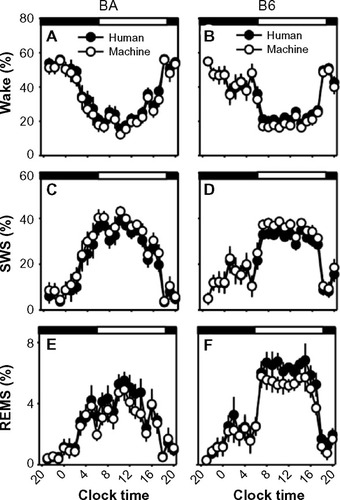
Table 2 Sleep states in 10-second epochs, human versus machine scoring (minutes/24 hours)

State	Strain	Human	Machine	ANOVA (scoring method)
Wake	BA	857±23	800±20	F1,20=40.0; P<0.001
	B6	819±15	780±18
SWS	BA	515±21	582±20	F1,20=37.6; P<0.001
	B6	529±14	583±16
REMS	BA	67±3	58±4	F1,20=54.0; P<0.001
	B6	91±3	78±4

Abbreviations: ANOVA, analysis of variance; BA, BALB/CJ mice; B6, C57BL/6J mice; REMS, rapid-eye-movement sleep; SWS, slow-wave sleep.

Figure 5 Sleep-state percentages in human-scored versus machine-scored 2-second epoch data.

Notes: Data from the BA strain (left column) and the B6 strain (right column) were binned into 12-minute intervals. Graphs represent the percentage of each interval spent in wake (A and B), SWS (C and D), and REMS (E and F). Open circles represent machine-scored data and filled circles represent human-scored data. Data are from Zeitgeber time 4–9.
Abbreviations: B6, C57BL/6J mice; BA, BALB/CJ mice; REMS, rapid-eye-movement sleep; SWS, slow-wave sleep.

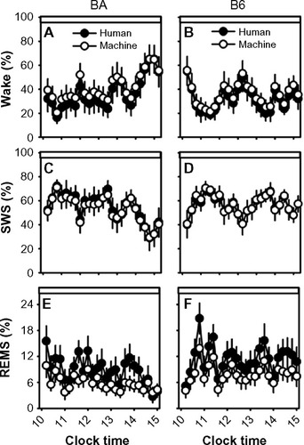
Figure 6 Machine-scored data in 10-second epochs exhibit similar frequency profiles to human-scored data.

Notes: The left column shows data for the BA strain and the right column shows data for the B6 strain. For wake (A and D), SWS (B and E), and REMS (C and F), the frequency profiles of the human-scored data (black line) and those of the machine-scored data (gray line) are shown. The black dots in panels (A, C, D and F) indicate frequency bands in which posthoc comparisons (Fisher’s protected least-significant difference) indicated a difference between the curves. The insets in panels (B and E) show 1–4 Hz SWA. P-values in these insets indicate main effect of scoring method on SWA.
Abbreviations: B6, C57BL/6J mice; BA, BALB/CJ mice; EEG, electroencephalography; EMG, electromyography; H, human; M, machine; NS, not significant; REMS, rapid-eye-movement sleep; SWA, slow-wave activity; SWS, slow-wave sleep.

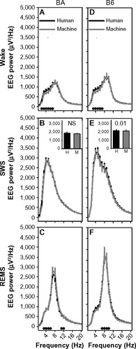
Figure 7 Homeostatic modeling of lactate data and SWA scored by human or machine.

Notes: The left column shows human-scored data and the right-hand column shows machine-scored data. The top four panels show scaled lactate data in 10-second epochs scored by a human (A), 10-second epochs autoscored (B), 2-second epochs scored by a human (C), and 2-second epochs autoscored (D). The bottom four panels show SWA in 5-minute sleep episodes using 10-second epochs scored by a human (E), 10-second epochs autoscored (F), 2-second epochs scored by a human (G), and 2-second epochs autoscored (H). In each panel, a homeostatic model for lactate or SWA was fit to the data (solid curve). The difference in time scale between the lower panels and the upper panels reflects the difference in temporal dynamics of SWA versus those of lactate.
Abbreviations: REMS, rapid-eye-movement sleep; SWA, slow-wave activity; SWS, slow-wave sleep.

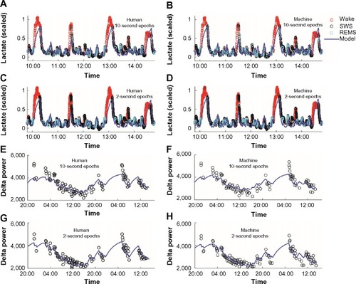
Figure 8 Strain differences in optimal time constants in general homeostatic modeling of state-dependent SWA and lactate dynamics.

Notes: Data represent optimized time constants for wake/REMS-dependent increases (τ_i) and SWS-dependent decreases (τ_d) in SWA (A–D) and lactate (E–H) from human-scored data (black bars) and machine-scored data (gray bars). P-values are shown for main effect of scoring method on time constants.
Abbreviations: B6, C57BL/6J mice; BA, BALB/CJ mice; NS, not significant; REMS, rapid-eye-movement sleep; SWA, slow-wave activity; SWS, slow-wave sleep.

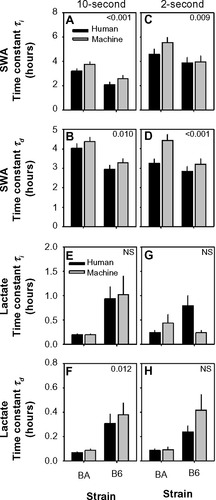
Figure 9 Differences in residuals of model fit to data scored by human or machine.

Notes: Data represent the residuals associated with optimized time constants for modeling SWA (A and B) and lactate (C and D) from human-scored data (black bars) and machine-scored data (gray bars) in either 10-second or 2-second epochs. P-values are shown for main effect of scoring method on time constants. Asterisk denotes significant difference for human versus machine scoring within the BA strain (Fisher’s protected least-significant difference).
Abbreviations: B6, C57BL/6J mice; BA, BALB/CJ mice; NS, not significant; R SWA, slow-wave activity.

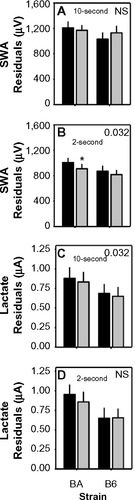
Table 3 Strain difference in sleep timing: human versus machine scoring

State	Method	BA versus B6, minutes/24 hours	ANOVA (strain)	ANOVA (strain × time)
Wake	Human	+38	NS	F1,20 =2.5; P<0.001
	Machine	+20	NS	F1,20 =2.5; P<0.001
SWS	Human	−14	NS	F1,20 =2.6; P<0.001
	Machine	−1	NS	F1,20 =2.6; P<0.001
REMS	Human	−24	F1,20 =27.0; P<0.001	F1,20 =2.5; P<0.001
	Machine	−20	F1,20 =12.0; P<0.002	F1,20 =2.5; P<0.001

Abbreviations: ANOVA, analysis of variance; B6, C57BL/6J mice; BA, BALB/CJ mice; NS, not significant; REMS, rapid-eye-movement sleep; SWS, slow-wave sleep.

Figure 10 Strain differences in sleep/wake state timing scored in 10-second epochs.

Notes: Strain differences in the time course of sleep/wake states were observed in human-scored data (A, C and E) or machine-scored data (B, D and F). Filled circles represent data from the BA strain, and open circles represent data from the B6 strain. Asterisks indicate 60-minute epochs in which there is a statistically significant difference between strains (Fisher’s protected least-significant difference). Timing of the dark and light phases of the 12:12 cycle is indicated by the black and white bars at the top of each graph.
Abbreviations: B6, C57BL/6J mice; BA, BALB/CJ mice; REMS, rapid-eye-movement sleep; SWS, slow-wave sleep.

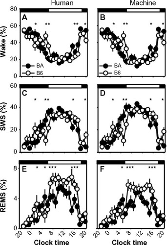
Figure 11 Strain differences in EEG power spectra in 10-second epochs scored by human or machine.

Notes: The left column shows human-scored data and the right column shows machine-scored data. For wake (A and D), SWS (B and E), and REMS (C and F), EEG power differed between strains at specific frequencies. The black dots at the base of each graph indicate frequency bands in which posthoc comparisons (Fisher’s protected least-significant difference) indicated a difference between the BA (black line) and B6 (gray line) strains. The insets in panels (B and (E) show 1–4 Hz SWA, which did not differ between strains.
Abbreviations: B6, C57BL/6J mice; BA, BALB/CJ mice; EEG, electroencephalography; NS, not significant; REMS, rapid-eye-movement sleep; SWS, slow-wave sleep.

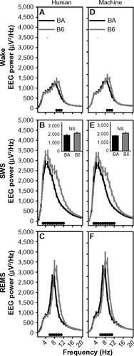
Table 4 Strain difference in 10-second EEG spectral profiles: human versus machine

State	Method	ANOVA (strain)	ANOVA (strain × frequency)
Wake	Human	NS	F19,380=4.3; P=0.001
	Machine	NS	F19,380=4.5; P=0.001
SWS	Human	F1,20=9.0; P=0.007	F19,380=7.9; P=0.001
	Machine	F1,20=9.0; P=0.007	F19,380=7.8; P=0.001
REMS	Human	NS	F19,380=12.8; P=0.001
	Machine	NS	F19,380=12.8; P=0.001

Abbreviations: ANOVA, analysis of variance; NS, not significant; REMS, rapid-eye-movement sleep; SWS, slow-wave sleep.

Table 5 Strain difference in homeostatic dynamics: human versus machine

Variable	Method	τi BA versus B6	τd BA versus B6
Ten-second
SWA	Human	τ20=3.7; P=0.001	τ20=3.3; P=0.003
	Machine	τ20=3.7; P=0.001	τ20=3.8; P=0.001
Lactate	Human	τ20=−3.1; P=0.005	τ20=−3.1; P=0.005
	Machine	τ20=−2.2; P=0.042	τ20=−3.0; P=0.006
Two-second
SWA	Human	τ20=1.2; NS	τ20=1.3; NS
	Machine	τ20=2.5; P=0.020	τ20=3.0; P=0.008
Lactate	Human	τ20=−2.5; P=0.019	τ20=−3.0; P=0.007
	Machine	τ20=−1.8; NS	τ20=−2.5; P=0.020

Abbreviations: B6, C57BL/6J mice; BA, BALB/CJ mice; NS, not significant; SWA, slow-wave activity.