
Figures & data
Table 1 Full Data Set, Training Set, Validation Set and External Data List
Figure 1 SAS and SAS_A scores demonstrated statistically significant differences between the two groups with and without disease progression (p < 0.0001) (A and B). ROC curve indicated that SAS_A could be used to differentiate disease progression events, with AUC = 0.684, 95% CI:0.627–0.742, p-value < 0.0001, cutoff value 53 (C). K-Ms survival study revealed a difference between the high and low SAS_A groups, with Log rank test p-value < 0.0001, median PFS: 50 months versus 17 months for the low and high score groups, HR (low versus high score groups):0.25 (0.16–0.60), relative risk reduction 75% (D). In the two groups with or without disease progression, there was a link between treatment SAS and SAS_A, but the correlation law was different (E), and the variation trend was inconsistent between SAS and SAS_A of patients (F).
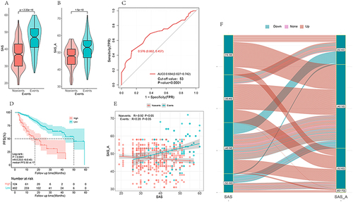
Figure 2 LASSO regression analysis and cross-validated Lasso regression analysis including all variables. When lambda was 1se and 2 variables (A and B) were included, variables were screened using the stepwise regression method and optimal subset (C and D), the relevance of each variable was screened using random forest (E), and a forest diagram of all variables was plotted (F). Different methodologies concentrated on the three aspects of SAS, income and family. To further compare the differences, we created model 3 with SAS, family, and income, and model 4 with all components.
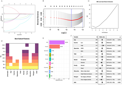
Figure 3 In the training set, the area under ROCA curve (AUC) was 0.665 (0.592–0.738) for model 1, 0.645 (0.567–0.723) for model 2, 0.668 (0.592–0.743) for model 3, and 0.696 (0.624–0.767) for model 4. In the verification set, the area under ROCA curve (AUC) was 0.654 (0.559–0.748) for model 1, 0.667 (0.584–0.770) for model 2, 0.673 (0.580–0.767) for model 3, and 0.712 (0.624–0.800) (A and F) for model 4. The calibration curve (B-J) was plotted to compare C index, Dxy index, Brier index, R2 (K) of different models in the training set and test set.
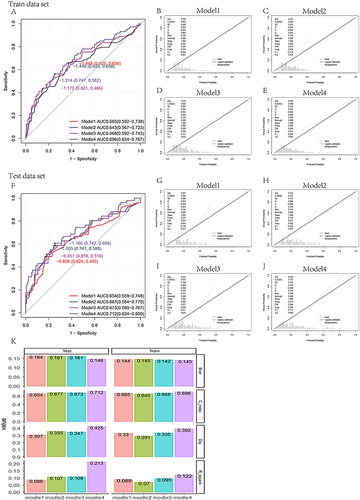
Figure 4 NRI of model 3 and model 4 was compared in the training set, test set and external dataset respectively. In the training set, the NRI between model 3 and model 4 was 0.0892 (−0.0351–0.2134), p = 0.15947. In the verification set, the NRI between model 3 and model 4 was 0.1529 (−0.0301–0.3359), p = 0.10142. In the external dataset, the NRI between model 3 and model 4 was 0.1529 (−0.0301–0.3359), p = 0.10142. In the external dataset, the NRI between model 3 and model 4 was 0.5368 (0.2899–0.7837), p < 0.001 (A-C). Calibration curve verification was performed for model 3 and model 4 in external datasets (D and E). The ROC curve (F) was plotted in the external dataset.
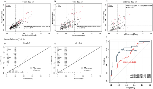
Table 2 A Score Table for Different Variables
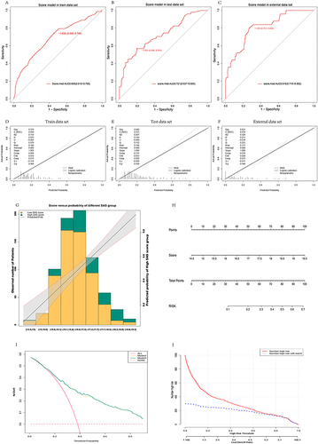
Figure 5 ROC was performed in training set, verification set and external data through score model after variable score conversion, and the results showed AUC 0.689 (0.618–0.760) in training set, AUC 0.721 (0.637–0.805) in verification set and AUC 0.810 (0.719–0.902) (A-C) in external data. Calibration curves (D-F) were plotted for the training set, test set and external data, respectively, and the distribution map was finally plotted for verification (G). The model was visualized by plotting nomogram (H). DCA curve found that model 3 and model 4 curves were both above the benefit curve with everyone intervened, which indicated that intervention of patients who are at high-risk by using the model could yield good clinical benefits. The two curves of model 3 and model 4 intertwined with each other and almost coincided, both of which yielded good clinical benefits (I). The CIC curve showed that as the predicted risk increased, the two curves gradually intersected, with predicted risks increasing and more anxiety state appearing (J).
Data Sharing Statement
All data generated or analysed during this study are included in this article. Further enquiries can be directed to the corresponding author.