Original endoscopic orbital decompression of lateral wall through hairline approach for Graves’ ophthalmopathy: an innovation of balanced orbital decompression

Figures & data

Figure 1 Decompression of lateral wall.

Notes: (A, B) “Three-point” incisions. ①=First cut; ②=second cut; ③=third cut. (a, b) Diagrammatic sketch of the “three-point” incisions. (C) The surgical field building. In the endoscopic vision through the second cut, ultrasonic scalpel and other auxiliary instruments were placed through the first cut and the third cut; ④,⑤=Surgical instruments. (c) Diagrammatic sketch of the surgical field building. (D) The lateral orbit wall exposure. Ultrasonic scalpel was used to cut about 3–4 cm² temporalis away behind the zygomatic process. The temporalis was moved away to expose the lateral orbit wall. The temporalis attached to the temporal fossa was cut through to avoid soft tissue depression after operation. ⑥=Bone of the lateral orbit wall in the fossae termporalis. (d, e, f) Diagrammatic sketch of the lateral orbit wall exposure. (E) Windowing of lateral wall of bone and fat. The electric grinding head was used to wear through the exposed lateral orbit bone wall and the orbital fat protruded sufficiently. ⑦=Orbital fat; ⑧=lateral orbit bone wall. (g) Diagrammatic sketch of the windowing of lateral wall of bone and fat. (F) Drainaging. Check the wound and find no active bleeding. Put the rubber membrane for drainaging at the orbit window and then close each cut. ⑨=Drainage strip. (h) Diagrammatic sketch of drainaging.

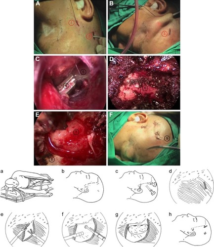
Figure 2 CT method used to assess the degree of proptosis.

Notes: “A” point to “B” point shows the interzygomatic line. “C” point to “D” point is the distance of protrusion. The arrows present the anterior margins of lateral bony orbital rim.
Abbreviation: CT, computed tomography.

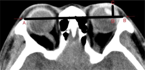
Figure 3 Postoperative stereogram of bone.

Note: The red triangle represents decompressed lateral bone wall.

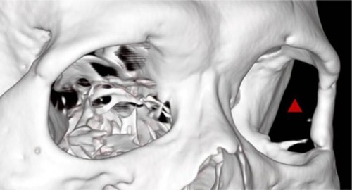
Table 1 The clinical data of surgery patients

No of patients	Age (years)	Sex	Side	Exophthalmometry (mm) (Hertel)		Visual acuity		IOP (mmHg)		sQOL-appearance
				Pre	Post	Pre	Post	Pre	Post	Pre	Post
1	20	F	L	19.50	17.00	0.6	0.6	21	19	37.50	43.75
2	34	F	L	23.50	20.00	0.8	0.8	22	22	62.50	75.00
3	53	M	R	20.50	16.00	0.4	0.6	24	15	50.00	68.75
4	71	F	L	20.00	16.50	0.8	0.8	20	16	37.50	62.50
5	23	M	R	24.00	20.00	1.0	1.0	17	14	50.00	68.75
6	52	F	L	20.50	16.00	1.0	1.0	20	17	43.75	75.00
7	51	M	R	19.00	17.00	0.25	0.3	20	21	50.00	68.75
8	51	M	L	22.00	17.00	0.5	0.6	23	21	25.00	31.25
9	51	M	L	18.00	16.00	0.6	0.6	18	18	50.00	56.25
10	44	M	L	26.00	22.50	0.1	0.1	26	18	50.00	62.50
11	49	F	R	16.50	13.00	0.8	0.8	21	22	62.50	62.50
12	42	M	L	18.00	13.00	1.0	1.0	20	18	31.25	43.75
13	28	M	L	21.50	17.00	0.6	0.7	20	18	37.50	68.75
14	40	F	L	21.00	17.00	1.0	1.0	18	16	68.75	87.50
15	20	F	R	18.50	15.50	0.25	0.5	24	16	43.75	62.50
16	43	M	L	23.00	18.50	1.0	1.0	18	19	50.00	75.00
17	61	F	R	18.00	14.50	CF/BE	0.1	25	17	56.25	81.25
18	30	M	R	17.50	14.00	1.0	1.0	18	18	50.00	75.00
19	61	F	L	25.00	19.00	0.6	0.8	24	18	56.25	75.00
20	51	M	R	22.00	17.00	0.3	0.5	15	16	31.25	62.50
21	47	F	L	19.50	15.50	0.8	0.8	14	13	56.25	68.75
22	58	F	L	22.00	18.00	HM/20 cm	0.3	26	21	43.75	75.00
23	33	M	R	17.00	13.50	1.0	1.0	19	20	68.75	87.50
24	53	F	L	22.50	18.00	1.0	1.0	19	18	50.00	81.25
25	35	M	R	22.00	17.00	1.0	1.0	21	19	37.50	68.75
26	50	M	L	27.00	20.00	1.0	1.0	23	21	31.25	50.00
27	28	M	L	22.50	18.00	0.2	0.4	18	18	37.50	62.50
28	37	F	R	23.50	18.50	0.1	0.1	16	17	43.75	62.50
29	44	M	R	26.00	22.00	0.1	0.1	18	17	37.50	75.00
30	37	F	R	25.50	18.00	0.5	0.6	20	19	18.75	62.50
31	58	M	L	15.00	10.50	0.5	0.5	21	17	62.50	87.50
32	50	F	L	15.50	12.00	0.6	0.8	22	14	62.50	81.25
33	37	F	L	21.00	17.00	0.8	0.8	19	17	50.00	75.00
34	24	F	L	21.50	17.50	HM/BE	0.1	17	14	6.25	50.00
35	30	M	R	18.00	14.50	0.6	0.6	18	18	50.00	75.00
36	30	F	L	19.00	14.00	0.8	0.8	15	15	56.25	93.75
37	26	F	L	20.00	17.00	1.0	1.0	18	17	56.25	68.75
38	52	F	L	19.50	14.50	0.25	0.3	14	14	43.75	87.50
39	49	F	L	19.00	14.00	0.8	0.8	21	18	50.00	68.75
40	25	F	R	18.00	13.50	0.5	0.5	17	17	50.00	75.00
41	42	F	R	19.00	16.00	HM/BE	HM/BE	20	15	37.50	87.50

Abbreviations: BE, blind eye; CF, counting fingers; F, female; HM, hand movement; IOP, intraocular pressure; L, left; M, male; R, right; sQOL, score of quality of life.

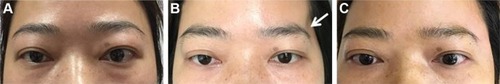
Figure 4 Postoperative appearance of patients.

Notes: (A) Appearance of preoperative; (B) appearance on first day after surgery; (C) appearance at 3 months after surgery. Left orbits of them were under operation. The above was anterior view, and below was head up 45° view.

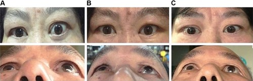
Figure 5 Reduction of proptosis obtained in 41 operations.

Notes: Proptosis was measured with Hertel’s exophthalmometry. ***P<0.0001.

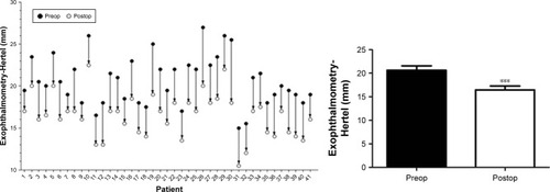
Figure 6 Reduction of proptosis obtained in 41 operations.

Notes: Proptosis was measured with CT method. ***P<0.0001.
Abbreviation: CT, computed tomography.

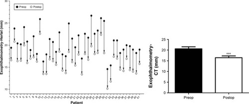
Figure 7 sQOL of visual function questionnaire.

Note: There is no significant difference.
Abbreviations: sQOL -VF, score of quality of life of visual function; ns, not significant.

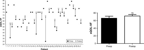
Figure 8 sQOL of appearance questionnaire.

Note: ***P<0.0001.
Abbreviation: sQOL-A, score of quality of life of appearance.

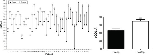
Figure 9 Overt depression of soft tissue at regions temporalis was rectified with autologous fat filling.

Notes: (A) The appearance at preoperation. (B) Overt depression of soft tissue at regions temporalis at 2 months after surgery (arrow); (C) repaired soft tissue depression.