Analysis of the metabolic properties of maintenance hemodialysis patients with glucose-added dialysis based on high performance liquid chromatography quadrupole time-of-flight mass spectrometry

Figures & data

Table 1 Demographics and clinical data of the subjects

	Control group	MHD group				Pre-HD P-value	Post-HD P-value
		G (−) group		G (+) group
		Pre-HD	Post-HD	Pre-HD	Post-HD
Number of cases (n)	10	10		10		/
Age (years)	49.1±15.2	53.3±18.6		51.1±13.2		0.33
BMI	23.6±2.2	24.1±3.5		23.7±3.1		0.56
Female (%)	50	40		30		0.12
DN as primary disease (%)	–	30		30		/
Kt/V	–	1.50±1.12		1.51±2.11		0.79
Dialysis time (months)	–	19.9±6.2		23.1±7.0		0.25
Hemoglobin (g/L)	133±12.3a	103±15.4		100±12.1		0.46
Blood indexes
Serum glucose (mmol/L)	4.83±0.53a	6.86±1.57	5.78±1.34	6.48±1.37	8.11±1.64	0.53	0.07
Serum K^+ (mmol/L)	4.41±0.35	5.54±0.89	3.20±0.96	5.38±0.79	3.47±0.52	0.37	0.42
Serum Na^+ (mmol/L)	141.52±3.91	138.83±6.32	139.07±5.99	136.44±3.92	139.32+4.77	0.58	0.81
Serum Ca^2+ (mmol/L)	2.34±0.17	2.36±0.18	2.40±0.24	2.35±0.17	2.39±0.21	0.81	0.2
Serum creatinine (μmol/L)	67.50±17.95a	913.49±291.51	296.70±57.72	948.81±302.19	312.78±60.89	0.56	0.51
BUN (mmol/L)	5.44±1.55a	26.91±7.82	9.27±3.13	27.74±7.49	9.98±3.45	0.41	0.42
Serum HCO3^− (mmol/L)	25.89±4.42	20.45±2.42	26.81±5.17	19.74±2.11	27.56±5.39	0.69	0.34

Note:

a Compared with the MHD group, P<0.05.

Abbreviations: BMI, body mass index; BUN, blood urea nitrogen; DN, diabetic nephropathy; HD, hemodialysis; G (−), glucose-free dialysate group; G (+), glucose dialysate group; Kt/V, (urea clear index); MHD, maintenance hemodialysis.

Figure 1 Base peak intensity chromatograms, using HPLC-MS/Q-TOF-MS, of plasma samples from: the G (−) group before hemodialysis (A), the G (+) group before hemodialysis (B), the G (−) group after hemodialysis (C), the G (+) group after hemodialysis (D), and the control group before hemodialysis (E).

Note: The G (−) group was treated with glucose-free dialysate, and the G (+) group was treated with glucose-added dialysate.
Abbreviations: HPLC, high performance liquid chromatography; MS, mass spectrometry; Q-TOF, quadrupole time-of-flight.

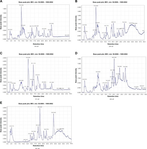
Figure 2 Principal component analysis score scatter plots (A) and orthogonal partial least squares–discriminate analysis score plots (B) based on plasma metabolic profiling of control patients and maintenance hemodialysis (G+, G−) patients before hemodialysis.

Key: 1, G (−) group; 2, G (+) group; 3, control group.

Notes: The G (−) group was treated with glucose-free dialysate, and the G (+) group was treated with glucose-added dialysate.

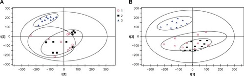
Figure 3 (A) Orthogonal signal correction–partial least squares discriminate analysis score plots of the three groups after hemodialysis. The ellipse shows the 95% confidence region for Hotelling’s T2 statistic for this model. Cumulative fitness (values) and prediction power (value) of this three-component model were 0.915 and 0.952, respectively. 1, G (−) group; 2, G (+) group; 3, control group. (B) Orthogonal partial least squares S-plot based on detected plasma metabolites from the G (−) and G (+) groups.

Notes: The G (−) group was treated with glucose-free dialysate, and the G (+) group was treated with glucose-added dialysate.

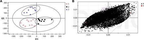
Figure 4 Identification procedure of the potential biomarker anandamide 0-phosphate. (A) The mass spectrum at the retention time of 7.10 minutes. (B) The MS/MS spectrum of the ion of m/z 225 at 7.10 minutes in the plasma sample. (C) The possible fragmentation mechanism of anandamide 0-phosphate.

Abbreviation: MS, mass spectrometry.

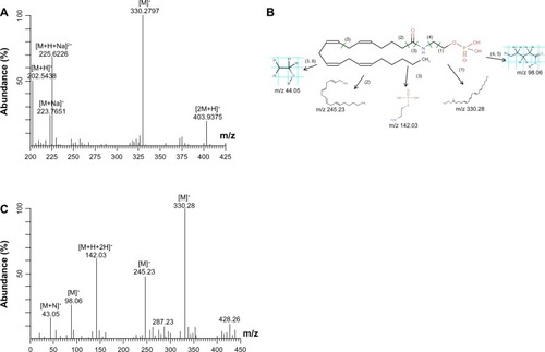
Table 2 Comparison of the main biomarkers in glucose and glucose-free dialysis

ID	m/z	RT	Tendency (↑/↓)	VIP	t-value	P-value	Name
1324	377	28:25	↓	5.3	3.35	0.026	Lithocholic acid
3476	371	29:10	↑	10.2	3.82	0.022	Dihydroxyprostaglandin F2α
34033	263	31:55	↑	4.7	3.25	0.030	Leucine
10418	271	35:30	↑	3.5	3.21	0.030	Unknown
8898	205	16:27	↓	4.4	3.14	0.031	Aspartate
10770	225	7:10	↓	6.6	3.00	0.032	Phosphorylated anandamide
33395	215	2:63	↓	3.8	2.65	0.040	Valine
57	746	15:75	↓	4.1	2.36	0.041	Unknown
13288	733	9:00	↑	7.9	2.18	0.044	Unknown

Abbreviations: ID, identification number; m/z, mass to charge ratio; RT, retention time; t, t value; VIP, variable importance projection.