Figures & data
Figure 1 The stacked rhombic dodecahedron alveolar sac model displayed from four different angles: an oblique view (A), a base view with a −15 degree x-axis rotation (B), a base view with a 15 degree x-axis rotation (C), and a base view with a 45 degree x-axis rotation (D).
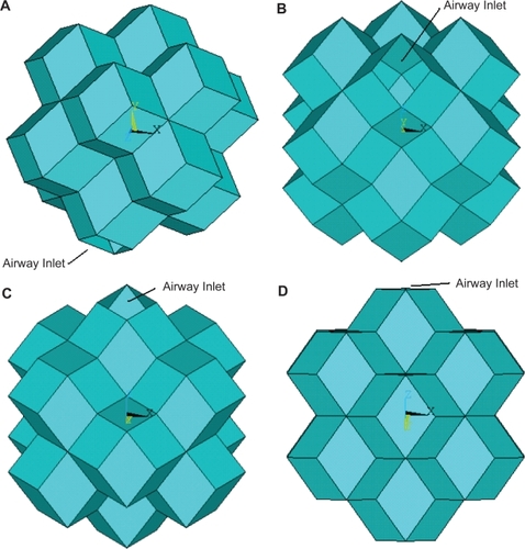
Table 1 The material properties for the eight lung volumes corresponding to normal conditions. The lung volumes are represented as percentages of total lung capacity (TLC). The stretch ratio reveals the length of the tissue after stretching compared with the resting state. The traction stress is used to apply the tethering forces for surrounding alveolar sacs and the young’s modulus reveals the increasing stiffness of the tissue as the lung volume increases
Figure 2 The Young’s modulus for the emphysematous and normal tissue for the featured lung volumes. The destruction of the collagen and elastin fibers in the emphysematous tissue decrease the strength and the elastic recoil of the tissue, hence reducing the Young’s modulus.
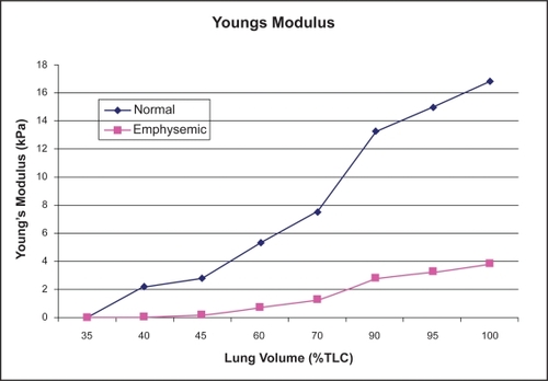
Figure 3 The stress distributions for the normal alveolar sac models at two different lung volumes. The low lung volume (A) and the high lung volume (B) reveal a very similar stress distribution.
Abbreviations: TLC, total lung capacity.
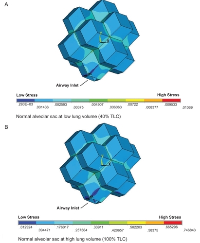
Figure 4 The stress distributions for the emphysematous alveolar sac models at two different lung volumes. A single area of the alveolar sac has the emphysematous material properties applied as highlighted in the figure. The low lung volume (A) and the high lung volume (B) reveal very different stress distributions. Specifically, very high stress levels are induced in the emphysematous area and the airway inlet at the low lung volume.
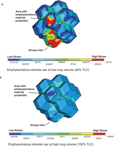
Figure 5 The external view of the alveolar sac model for the different disease states investigated at a mid lung volume of 60% total lung capacity. The states were: normal conditions (A), normal material properties with an elevated internal pressure (B), one simulated emphysematous alveolar wall with normal pressure (C), and finally a simulated emphysematous wall and elevated internal pressure (D). It can be seen from these external views that the stress distribution on the outer wall is disrupted for both emphysema models.
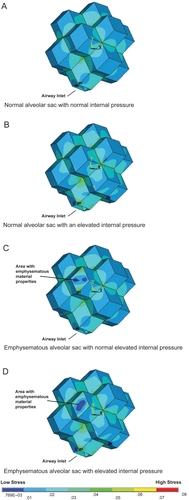
Figure 6 The internal view of the alveolar sac model at a lung volume of 60% total lung capacity showing the model sliced through the medial plane to reveal the inner wall of the emphysematous area. The states illustrated are: normal conditions (A), normal with an elevated internal pressure (B), a simulated emphysematous alveolar wall with normal pressure (C), and finally a simulated emphysemic wall and elevated internal pressure (D). These internal views highlight the elevated stress through out the internal emphysematous wall, with particularly high stresses at the wall junction sites.
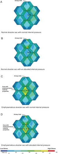
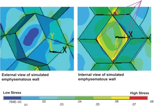
Figure 7 A close up view of the simulated emphysematous wall incorporating the elevated internal pressure. Highlighted, is the significantly elevated stress levels at the internal junctions with the adjoining alveolar walls.