Figures & data
Figure 1 A 32-segment quadric fractal. The basic pattern shown in the upper box can be seen repeated throughout the structure at different scales. When the figure is viewed at a scale factor of 8 relative to the previous view, the pattern repeats itself with 32 pieces, each 1/8 the length of the original of which it is a part.
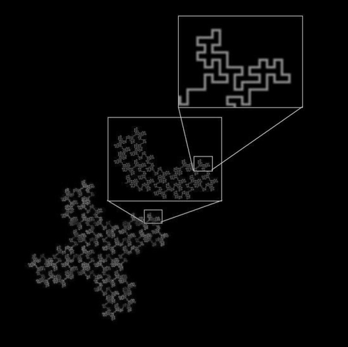
Figure 2 Calculating the local connected fractal dimension (Dconn). Each pixel, P(x, y), that represents part of the vascular tree in a retinal vessel image has an associated local connected set for every distance that can be defined around that pixel. As illustrated at the bottom left of the figure, the local connected set includes only the pixels that can be traced along a continuous path from P(x, y). As illustrated at the bottom right, this set is used to calculate the Dconn at (x, y). The image shows the data gathering process in which concentric squares of decreasing size are laid on the connected set and a local dimension is determined accordingly (see text).
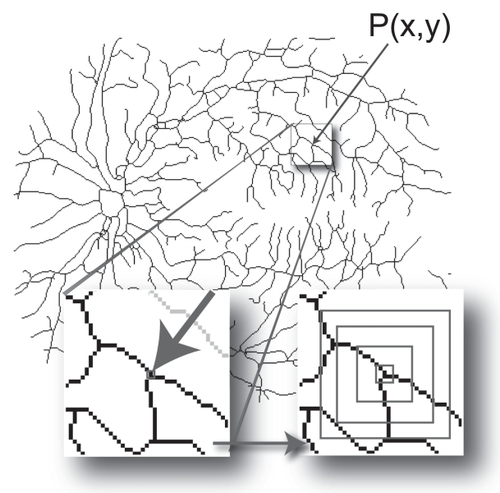
Figure 3 The range for area under the curve (AUC) was between 0.7185 to 0.9492, with an average and standard deviation of 0.8832 ± 0.0397. The accuracy values average and standard deviation was 0.903 ± 0.018.
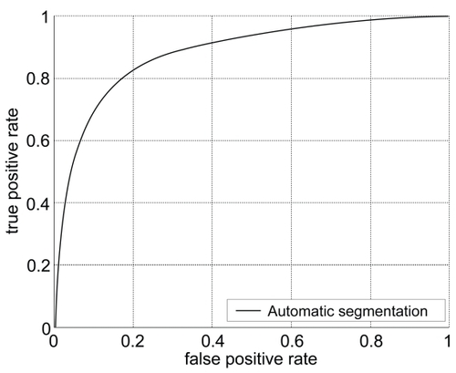
Figure 4 Results of the box-counting analysis and the local connected dimension analysis using all 27 images, for the manually segmented group and the automatically segmented group. Image names prefaced by PDR are the proliferative retinopathy images, and images with no letter in front are the control images. Box Counting: The figure shows the global box counting dimension (DB) for each image. Local Connected Dimension: The figure shows the mean local connected fractal dimension (μDconn) for each image, calculated by averaging the Dconn values for each pixel in each image.
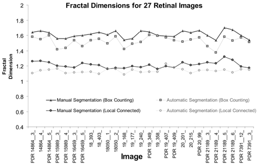
Figure 5 Noise affected automated segmentation. Shown here are two original fluorescein images (bottom) and their respective segmented and skeletonised vessel patterns (top). In image 16459__3_ on the left, fluorescein was relatively evenly distributed and the two patterns yielded similar global DBs (automated = 1.54 and manual = 1.59; see also). In image 20_201_ on the right, however, fluorescein was unevenly distributed, which caused some areas that were traced in the manual group to be left blank in the automated group, and the global DBs consequently differed more (automated 1.52 and manual = 1.66).
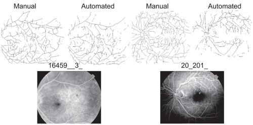
Figure 6 Automated segmentation of a retinal blood vessel pattern. A. The original fluorescein labeled image 18_393__. B. The automatically segmented and skeletonised vascular pattern from the image. C. The automatically segmented pattern from B, dilated to a uniform diameter and shown overlain on the original image as a dark vessel pattern over the fluorescein-labeled (white) vessels to illustrate the correspondence of the automatically selected pattern with vessels in the original.
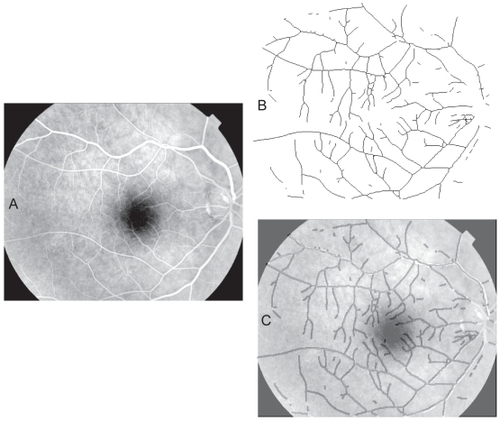
Table 1a Results of t-tests for automatically segmented images
Table 1b Results of t-tests for manually segmented Images
Figure 7 The distribution of the μDconn per image for all automatically segmented images. The group of PDR images, which were more severely pathological, had a significantly higher μDconn (see ).
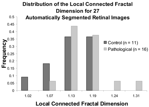
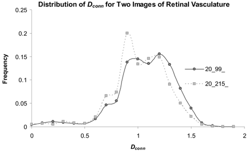
Figure 8 Distributions of the Dconn per pixel for two automatically segmented images. The μDconn values for the two patterns were significantly different (image 20__99_ = 1.10 ± 0.14 ; image 20__215 = 1.14 ± 0.15; p = 0.02); in addition, the distributions highlight specific areas where the Dconn per pixel varied.