
Figures & data
(A) High-resolution, static, black-blood imaging to evaluate thoracic and cardiovascular anatomy. (B) Dynamic (CINE) white-blood imaging (balanced steady-state free precession) of the left ventricular short- and long-axis to assess regional and global cardiac function. (C) Contrast enhanced perfusion imaging to confirm contrast injection. (D) Post-contrast static late gadolinium enhancement for evaluating myocardial fibrosis (white arrows).
CINE: Dynamic image; LGE: Late gadolinium enhancement.
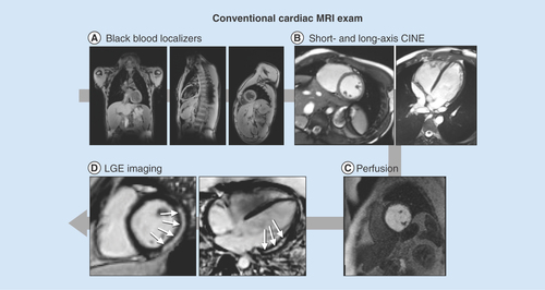
Table 1. Age and measures of left ventricular mass and function in normal healthy boys and boys with Duchenne muscular dystrophy.
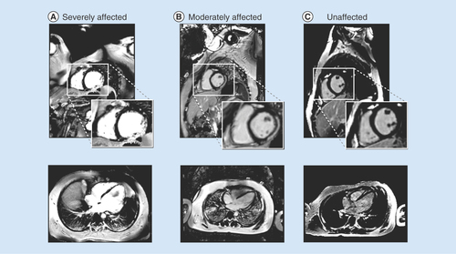
(A) A boy with Duchenne muscular dystrophy and strong cardiac involvement; (B) a moderately affected boy with moderate cardiac involvement and (C) a healthy volunteer with no signs of fibrosis.
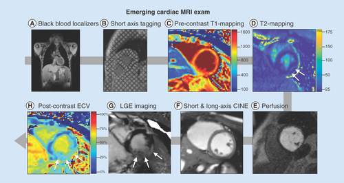
(A) High-resolution, static, black-blood imaging to evaluate thoracic and cardiovascular anatomy (B) short and long axis tagged images for the computation of cardiac strain and twist, (C & H): pre- and post-contrast T1 mapping and extracellular volume for the assessment of cardiac structural changes, (D) perfusion imaging to ensure contrast injection, (E) T2 mapping and apparent diffusion coefficient images for the assessment of cardiac structural changes, (F) dynamic (CINE) white-blood imaging (balanced steady-state free precession) of the left ventricular short and long axis to assess regional and global cardiac function and (G) post-contrast static late gadolinium enhancement for evaluating myocardial fibrosis.
CINE: Dynamic images; ECV: Extracellular volume; LGE: Late gadolinium enhancement.
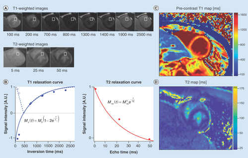
(A) A series of cardiac images are acquired at different times after an ‘inversion pulse’ that manipulates the longitudinal magnetization and the corresponding image contrast. Alternately, in (B) a series of images are acquired after different durations of ‘T2 preparation’ that manipulates the transverse magnetization and the corresponding image contrast. (B) Curve fitting is performed on a pixel-wise or region of interest basis (white boxes) and used to estimate the local tissue’s T1 and T2. The signal intensities (dots) represent the relative magnitude of the magnetization used to produce each of the images. Solid curves represent the curve fit for the equation in each plot. Additionally, the T1 plot shows the dashed curve with the first few data points not inverted about the ‘null-point’ – where signal from myocardium is suppressed (∼700 ms). After curve fitting (C) T1- and (D) T2-maps are generated on a pixel-wise basis.
By analyzing the deforming tag patterns between (A) diastole and (B) systole, it is possible to create (C) regional quantitative circumferential strain maps. Left ventricular strain describes how a (D) ‘reference’ region (gray circle) in diastole deforms via circumferential shortening (dashed line) and radial thickening (solid line) at peak systole.
DMD: Duchenne muscular dystrophy.
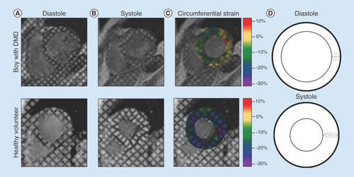
Table 2. Age and measures of left ventricular regional function in normal healthy boys and boys with Duchenne muscular dystrophy.
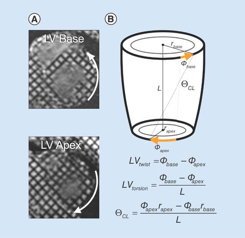
(A) MRI tagging at the base and apex can be used to estimate left ventricular rotational mechanics, including (B) left ventricular twist, torsion and CL shear (θCL).
LV: Left ventricular; CL: Circumferential–longitudinal.