Figures & data
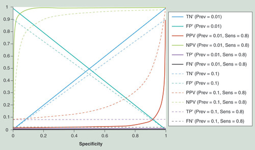
Shown are assay outcomes for a given sensitivity of 0.8 and two values of disease prevalence (0.1 and 0.01, respectively) plotted against assay specificity. Assay outcomes are TN’ (i.e., the number of TNs divided by the total number tested), FP’, TP’, FN’, PPV (i.e., the number of TPs divided by the total number of positive tests, which corresponds to the probability of having the disease if tested positive), and NPV (i.e., the number of TNs divided by the total number of negative tests). The graph shows clearly the strong dependency of PPV on prevalence, and its rapid decline with decreasing specificity.
FN’: False-negative proportion; FP’: False-positive proportion; NPV: Negative predictive value; PPV: Positive predictive value; Prev: Prevalence; Sens: Sensitivity; TN’: True-negative proportion; TP’: True-positive proportion.
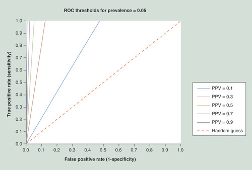
PPV can be described as a function of specificity, Sens and Prev as shown in the figure. However, the PPV may be approximated for small Prev (Prev <1) as a function of specificity and a constant (Sens*Prev). Hence, for a given (constant) Prev, the curves each correspond to a particular level of Sens. During assay development, such a graph can be used to define target specificity and Sens of the biomarker panel when a certain PPV value has to be reached (in order to confer clinical utility): For example, one could first define a range of Sens deemed realistic (e.g., 0.2–1.0; to also cover the most optimistic case). These values, multiplied with the Prev, result in the set of (Sens*Prev) curves, which delimit the specificity range one has to aim for. A horizontal line may be drawn between those curves at the desired PPV, and the intersection between the line and the curves is used to look up the specificity needed for different Sens. Importantly, the horizontal line becomes much shorter and moves to the right with increasing PPV (since it always has to connect the same set of [Sens*Prev] curves for a given Prev and specificity range; e.g., see B & C). This illustrates the strong dependency upon Prev (i.e., how the required specificity increases drastically with lower prevalence, even when a broad range of Sens is allowed). Three examples for this approach are given (A, B & C); the estimated and exact specificity values for these examples are shown in the table. (The Prev numbers given for ovarian and breast cancer are arbitrary and only for illustration; see text for discussion on cancer epidemiology.).
†Estimated assuming prevalence <1.
PPV: Positive predictive value; Prev: Prevalence; Sens: Sensitivity.
![Figure 2. Approximating clinical assay characteristics for prevalencePPV can be described as a function of specificity, Sens and Prev as shown in the figure. However, the PPV may be approximated for small Prev (Prev <1) as a function of specificity and a constant (Sens*Prev). Hence, for a given (constant) Prev, the curves each correspond to a particular level of Sens. During assay development, such a graph can be used to define target specificity and Sens of the biomarker panel when a certain PPV value has to be reached (in order to confer clinical utility): For example, one could first define a range of Sens deemed realistic (e.g., 0.2–1.0; to also cover the most optimistic case). These values, multiplied with the Prev, result in the set of (Sens*Prev) curves, which delimit the specificity range one has to aim for. A horizontal line may be drawn between those curves at the desired PPV, and the intersection between the line and the curves is used to look up the specificity needed for different Sens. Importantly, the horizontal line becomes much shorter and moves to the right with increasing PPV (since it always has to connect the same set of [Sens*Prev] curves for a given Prev and specificity range; e.g., see B & C). This illustrates the strong dependency upon Prev (i.e., how the required specificity increases drastically with lower prevalence, even when a broad range of Sens is allowed). Three examples for this approach are given (A, B & C); the estimated and exact specificity values for these examples are shown in the table. (The Prev numbers given for ovarian and breast cancer are arbitrary and only for illustration; see text for discussion on cancer epidemiology.). †Estimated assuming prevalence <1.PPV: Positive predictive value; Prev: Prevalence; Sens: Sensitivity.](/cms/asset/8e2cacc2-06f6-463e-9dc1-7a74c85e044d/iepi_a_12324903_f0002.jpg)
The characteristics of any biomarker assay can be drawn into this plot with a receiver-operating characteristic curve, and then used to determine the PPV that can be reached with this assay, and the sensitivity and specificity to which the assay has to be set; only when the receiver-operating characteristic curve is partially located to the left of a particular PPV threshold can that PPV be achieved.
PPV: Positive predictive value.
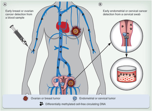
(A) Cell-free circulating tumor DNA from a blood sample for detection of breast and ovarian cancers from which tissue cannot be obtained readily; and (B) tumor DNA from vaginal fluid for the detection of endometrial and cervical cancers.
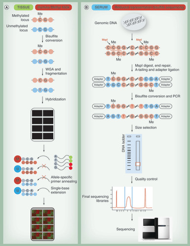
(A) For the Illumina Methyl 450K array, DNA is treated with bisulfite to convert all unmethylated cytosines into uracil. During subsequent whole-genome amplification, uracil is replaced by thymine. DNA is randomly sheared; fragmented DNA is loaded onto the chip and hybridizes to either methylated (M) or unmethylated (U) probes. Binding of methylated loci to methylated probes leads to single base extensions and fluorescently tagged nucleotides. Analogously unmethylated loci bind to unmethylated probes. Finally, the proportion of incorporated fluorescent nucleotides is quantified for each probe. (B) Reduced representation sequencing enriches DNA for CpG rich regions by cleavage using a restriction enzyme (e.g., MspI being most commonly used). After enzymatic digestion, the ends of DNA fragments are repaired (filled with nucleotides) and sequencing adapters are ligated. Subsequently, the adapter-ligated DNA is bisulfite-converted and amplified by PCR. Subsequent size selection by agarose gel electrophoresis ensures that only fragments having the restriction site (‘CCGG’ for MspI) on both ends within a small nucleotide range are sequenced. The DNA is extracted from gel, quality is controlled and the libraries are sequenced. By comparison of the sequence reads to a genomic reference, methylation rate for each cytosine present in the libraries is determined.
WGA: Whole-genome amplification.
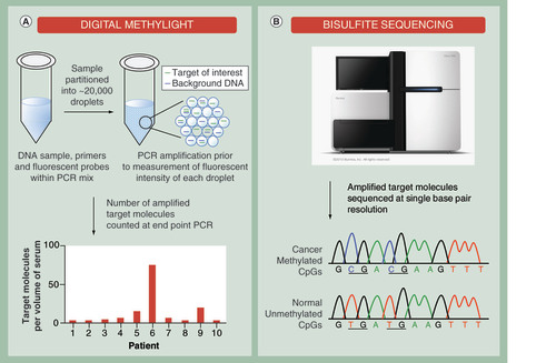
(A) Analysis of bisulfite-modified cell-free DNA by digital PCR. Each individual sample is partitioned into 1000s of nanoliter partitions via oil emulsion and dispersion. Low abundant cancer-specific and differentially methylated targets are sequestered away from wild-type background DNA to increase the signal-to-noise ratio. The absolute number of target molecules is counted at end point PCR and expressed as number of molecules per volume of serum allowing patient samples to be compared. (B) Bisulfite sequencing of cell-free DNA derived from serum. Following bisulfite conversion, specific DNA regions that are aberrantly methylated in cancer samples can be analyzed at single base-pair resolution.
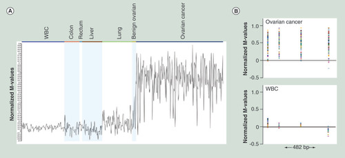
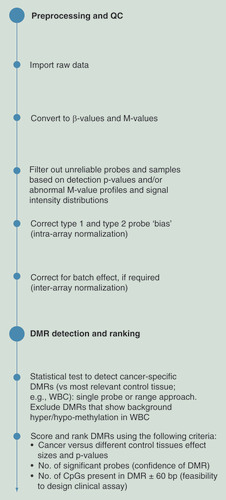
After the preprocessing and QC, DMR detection is carried out by comparing the methylation of cancer and WBC samples. After DMR detection, several steps and criteria are applied for filtering and ranking.
DMR: Differentially methylated region; QC: Quality control; WBC: White blood cell.
Data from Illumina 450K arrays is shown. (A) Normalized M-value profiles (arithmetic mean of the probes within the range) for all the relevant samples. (B) Normalized M-values of individual probes in the genomic context for ovarian cancer and WBC samples; 482 bp genomic region with four probes is shown.
WBC: White blood cell.