Figures & data
Figure 1. Pure-tone audiometry results of the two cases, first and second electric acoustic stimulation (EAS) in the left and right ear, respectively. Each hearing level threshold was determined preoperatively, and postoperatively after 1, 3, 6, and 12 months.
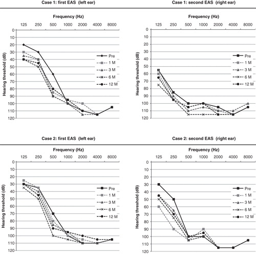
Figure 2. Japanese alphabetical monosyllable, word, and sentence scores at 1 year after fitting. Speech sound was presented at 65 dB SPL in quiet for monosyllable only and at +10 dB signal-noise ratio (SNR) for monosyllable, word, and sentence. These bar graphs show three conditions: (1) using the first electric acoustic stimulation (EAS) (implanted in the left ear in both cases), (2) using the second EAS (implanted in the right ear in both cases), and (3) using the bilateral EAS.
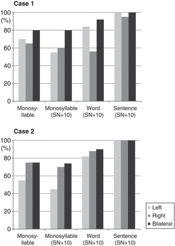
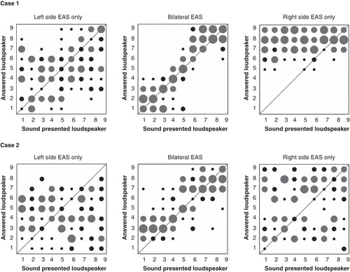
Figure 3. The scatter diagram shows the sound localization test results of the two cases. The horizontal axis shows the number of surrounding speakers from –90° to 90° azimuth, and the vertical axis shows the number of speakers that the patient answered correctly. Speaker no. 5 was directly in front of the patient. The size of each circle in the diagram indicates the number of times the patient chose each specific speaker. Larger circles show that the patient chose a speaker more frequently, while smaller circles indicate less frequently chosen speakers. The position of each circle indicates the position of the presented speaker that the patient chose.