A feasibility study for non-invasive thermometry using non-linear ultrasound

Figures & data

Figure 1. Comparison between a linear and a non-linear pulsed, plane acoustic wave. The waves propagate in water and are evaluated at a propagation distance x = 0.1 m; (A) temporal results, (B) spectral results. The non-linear waves are obtained by using the solution of the Burgers equation.

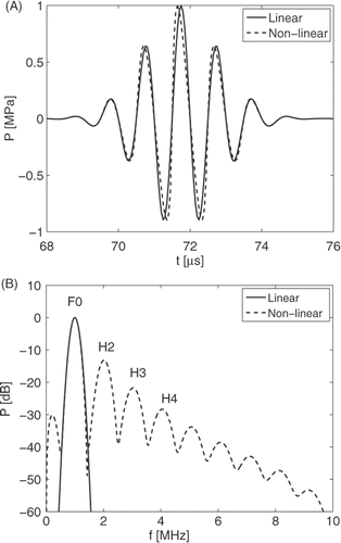
Figure 2. The one-dimensional transmission-mode set-up used for demonstrating the non-invasive thermometry method. An electric pulse drives a submerged acoustic transducer S which generates an acoustic wave field. The non-linearly propagating field is measured with a receiver R. The received analogue signal is converted via an A/D converter and recorded by the computer for further signal processing.

Figure 3. Acoustic medium parameters of water as a function of temperature, at ambient pressure; (A) specific heat c_p, (B) volume density of mass ρ, (C) volume coefficient of thermal expansion α_T, (D) acoustic absorption coefficient . Continuous results (solid lines) are obtained by interpolating discrete values (dots). The values are obtained from Lide, Spickler et al., and Wilson [49–51].

Figure 4. The speed of sound of water as a function of pressure and temperature. The values are obtained from the model by Wilson [51].

Figure 5. The contributions to the acoustic non-linearity parameter B/A of water arising from isothermal pressure changes and isobaric temperature changes, at ambient pressure.

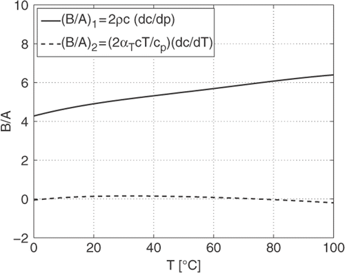
Figure 6. The computed acoustic non-linearity parameter B/A of water at ambient pressure, compared with values obtained by Beyer [44] and Hagelberg et al. [54].

Figure 7. The relative changes of the parameters B/A, c, ρ, , , and c_p of water. The reference temperature is T = 37°C at ambient pressure.

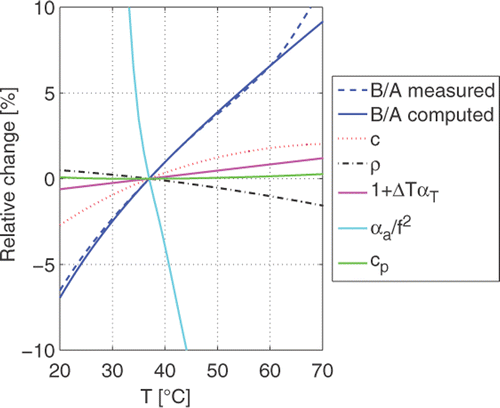
Table I.  The relative changes of the parameters B/A, c, ρ, α_T, , and c_p when T increases from 37°C to 42°C and from 37°C to 70°C, for water.

Parameter	Value			% change
	T = 37°C	T = 42°C	T = 70°C	37°C → 42°C	37°C → 70°C
B/A (computed)	5.41	5.50	5.91	1.6%	9.1%
c	1524 m/s	1532 m/s	1555 m/s	0.6%	2.0%
ρ	993.3 kg/m^3	991.4 kg/m^3	977.8 kg/m^3	−0.2%	−1.6%
1 + ΔT αT	1.000	1.002	1.012	0.2%	1.2%
αa/f ^2	1.35 · 10^−16 s^2/cm	1.26 · 10^−16 s^2/cm	0.70 · 10^−16 s^2/cm	−6.9%	−48.3%
cp	4178 J/(kg K)	4179 J/(kg K)	4190 J/(kg K)	0.005%	0.264%

Figure 8. Plane acoustic wave at a propagation distance x = 0.1 m in glycerol at temperatures T = 40°C, 50°C, 60°C; (A) temporal results, (B) spectral results, normalised with respect to the fundamental F₀.

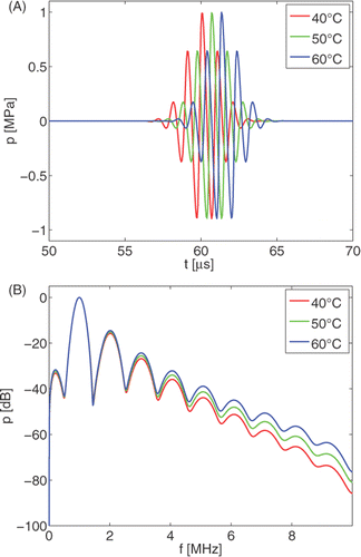
Figure 9. Simulated measurement data for a plane acoustic wave in glycerol, as computed with the solution of the Burgers equation and contaminated with 1% white noise; (A) temporal results, (B) spectral results for several different situations.

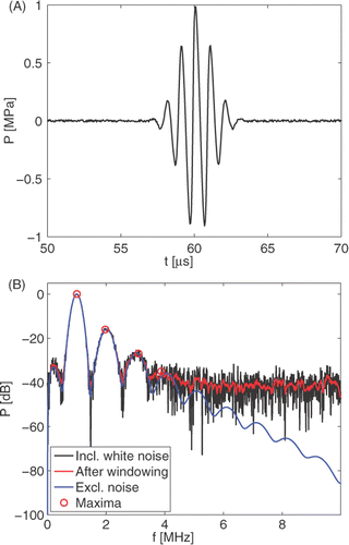
Figure 10. Comparison of the temperature dependent reference ratios (blue lines) and the measurement ratios obtained from the simulated measurement data (red lines). The simulated measured ratios are obtained from the single simulated measurement in Figure 9.

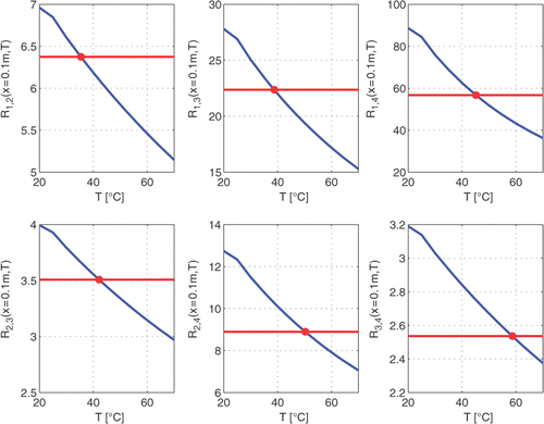
Figure 11. Prediction of the temperature from the single simulated measurement in Figure 9; (A) employing the fundamental, second and third harmonic, (B) employing the fundamental, second, third and fourth harmonic. The blue dots indicate the temperature obtained from the comparison of the individual simulated measurement and reference ratios. The red stars give the average temperature, and the red lines show the standard deviation.

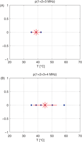
Table II.  Predicted temperatures from simulated measurements in glycerol. The temperature to be reconstructed is T = 40°C. In the notation , μ is the mean and σ the standard deviation of the averaged predictions.

Ratios involved	Single simulated measurement	16 simulated measurements
R1,2	35°C	40 ± 2°C
R1,2, R1,3, R2,3	39 ± 3°C	44 ± 3°C
R1,2, R1,3, R2,3, R1,4, R2,4, R3,4	45 ± 8°C	–

Wilson WD. Speed of sound in distilled water as a function of temperature and pressure. J Acoust Soc Am 1959; 31: 1067–1072

 Web of Science ®Google Scholar

Beyer RT. Parameter of nonlinearity in fluids. J Acoust Soc Am 1960; 32: 719–721

 Web of Science ®Google Scholar

Hagelberg MP, Holton G, Kao S. Calculation of B/A for water from measurements of ultrasonic velocity versus temperature and pressure to 10 000 kg/cm2. J Acoust Soc Am 1967; 41: 564–567

 Google Scholar