Figures of merit and their bounds in radiofrequency heating by phased arrays

Figures & data

Figure 1. Array of antennas radiating onto a body Ω as a multiport microwave junction. ω is the target. Waves entering and leaving the junction are also shown.

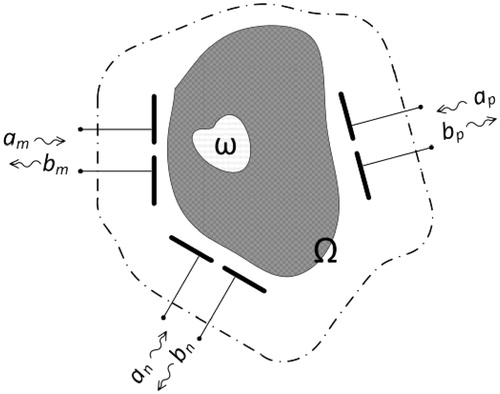
Figure 2. Eigenvalues μ₁ and μ₂ for a two-element array in front of a layered phantom (also shown in the inset) versus dipole spacing s. Depending on input setting [a], feed efficiency η_F takes values in the dashed area between the μ₁, μ₂ curves.

Figure 3. Planar multilayer phantom: w_s = 4 mm, w_f = 10 mm, w_b = 20 mm, w_c = 50 mm. A cube target with side 34.2 mm is also shown.

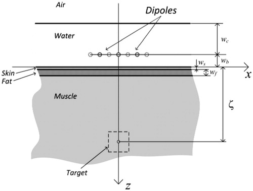
Table I. Physical parameters.

	ϵr	σe (Sm^−1)
Muscle	57	0.80
Fat	5.6	0.04
Skin	46	0.70
Distilled water	80	0.04

Figure 4. 11-element planar array. Row spacing d and dipole spacing s are free parameters in the numerical analysis.

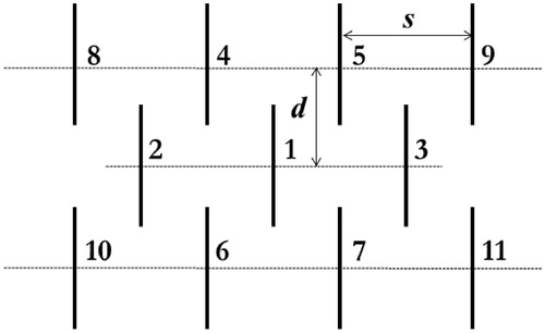
Figure 5. Smallest eigenvalue, μ_min, of matrix [H] versus s and d.

Figure 6. (A) λ_max, and (B) ν_max versus s and d.

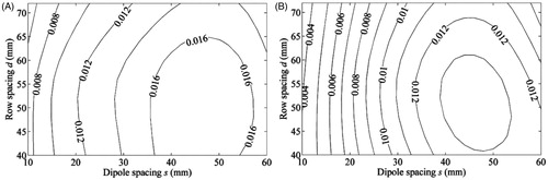
Figure 7. Relative array factor g_H as a function of s and d.

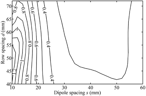
Figure 8. β_T versus s and d, (A) for ζ = 60 mm, (B) for ζ = 40 mm. α = 0.0186 mm^-1.

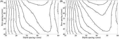
Figure 9. (A) Sagittal and (B) transverse images from the Visible Human Project (male). A cylindrical tumour and a water bolus containing the dipoles are included.

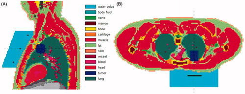
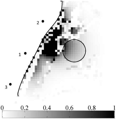
Figure 10. Power deposition (mW/cm³) in the sagittal plane through the tumour centre, for P_Ω = 1 W. Skin–bolus interface and tumour border are marked by solid lines. P_d,max= 10 mW/cm³. Dipoles 1–3 are also shown.