Figures & data
Table I. Selected kinetic coefficients, μ, for relative reaction rates, Equation (3) [Citation29].
Table II. Collected representative Arrhenius kinetic coefficients for heating processes.
Figure 1. Loss of clonogenicity curve for asynchronous Chinese hamster ovary (CHO) cells (triangles) compared to an Arrhenius prediction (solid line) with A = 2.84 × 1099 (s−1), and Ea = 6.18 × 10⁵ (J mol−1), () as derived from the constant rate regions of the original data [Citation20]. The shoulder region lasts for the first 60 min in this measurement. The Arrhenius prediction (straight line) substantially overestimates the cell death rate. A 50% loss of clonogenicity occurs at about 32 min in the experimental data, asynchronous cells are shown. An additional probabilistic model, presented by Mackey and Roti Roti [Citation16] is also shown (to be discussed in a later section). The probabilistic model separates G1-phase (—) and S-phase (— - —) CHO cells.
![Figure 1. Loss of clonogenicity curve for asynchronous Chinese hamster ovary (CHO) cells (triangles) compared to an Arrhenius prediction (solid line) with A = 2.84 × 1099 (s−1), and Ea = 6.18 × 10⁵ (J mol−1), (Table II) as derived from the constant rate regions of the original data [Citation20]. The shoulder region lasts for the first 60 min in this measurement. The Arrhenius prediction (straight line) substantially overestimates the cell death rate. A 50% loss of clonogenicity occurs at about 32 min in the experimental data, asynchronous cells are shown. An additional probabilistic model, presented by Mackey and Roti Roti [Citation16] is also shown (to be discussed in a later section). The probabilistic model separates G1-phase (—) and S-phase (— - —) CHO cells.](/cms/asset/9842d7e3-1483-4a56-8a2e-5e0d35318d63/ihyt_a_786140_f0001_b.jpg)
Figure 2. Simplified caspase feedback control block as used in the numerical models of apoptosis [Citation19] tBid is truncated (cleaved) Bid, which enters the mitochondrial inter-membrane space and releases cytochrome c and Smac/DIABLO. The many inhibiting inputs (i.e. BAR) have been eliminated for clarity. Other unused proteins are also sent for degradation (not shown in this figure).
![Figure 2. Simplified caspase feedback control block as used in the numerical models of apoptosis [Citation19] tBid is truncated (cleaved) Bid, which enters the mitochondrial inter-membrane space and releases cytochrome c and Smac/DIABLO. The many inhibiting inputs (i.e. BAR) have been eliminated for clarity. Other unused proteins are also sent for degradation (not shown in this figure).](/cms/asset/a4d601c7-9e1e-4141-8ebb-f9e6b15dacf8/ihyt_a_786140_f0002_b.jpg)
Figure 3. Model calculations of the dynamic response of the C3* output to input signal strengths (C8*) at 750 and 3000 molecules/cell [Citation19]. Copasi 4.8 was used to make the calculations based on a model file kindly provided by Thomas Eissing.
![Figure 3. Model calculations of the dynamic response of the C3* output to input signal strengths (C8*) at 750 and 3000 molecules/cell [Citation19]. Copasi 4.8 was used to make the calculations based on a model file kindly provided by Thomas Eissing.](/cms/asset/2484e1e7-9075-49a8-8c31-6528c68c13e4/ihyt_a_786140_f0003_b.jpg)
Figure 4. (A) Plot of the stochastic response of a population of cells. (B) Plot of the probability density function (pdf) impressed on the strength of the input signal, C8*, that resulted in part (A) response [Citation19].
![Figure 4. (A) Plot of the stochastic response of a population of cells. (B) Plot of the probability density function (pdf) impressed on the strength of the input signal, C8*, that resulted in part (A) response [Citation19].](/cms/asset/60088b37-9ffa-4717-9907-4a07b329641a/ihyt_a_786140_f0004_b.jpg)
Figure 5. Sketch of the shift of a population of G1 phase CHO cells in the probabilistic model of Mackey and Roti Roti as temperature increases from an initial 37 (εm = 0) to εm = −5 at 43 °C after a long time [Citation16].
![Figure 5. Sketch of the shift of a population of G1 phase CHO cells in the probabilistic model of Mackey and Roti Roti as temperature increases from an initial 37 (εm = 0) to εm = −5 at 43 °C after a long time [Citation16].](/cms/asset/1c3894e6-2659-4032-9036-55a432565c56/ihyt_a_786140_f0005_b.jpg)
Figure 6. Feng et al. [Citation18] prediction of the survival curve at 44 °C for PC3 cells (solid line) and an Arrhenius fit based on coefficients derived from the constant-rate region of the ensemble of experiments (dashed line).
![Figure 6. Feng et al. [Citation18] prediction of the survival curve at 44 °C for PC3 cells (solid line) and an Arrhenius fit based on coefficients derived from the constant-rate region of the ensemble of experiments (dashed line).](/cms/asset/d141f888-744f-4da9-9ee5-9ed0c16840da/ihyt_a_786140_f0006_b.jpg)
Figure 7. Comparison of numerical model and experimental surface temperature measurements for a tissue thickness of 1 mm at the beam centre (solid line/squares) and at the ±1σ beam radius (dashed line, open circles/triangles).
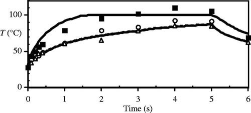
Figure 8. Tm:YAG laser thermal damage fields at t = 8 s. All four contours represent 63% damage (Ω = 1) for each damage process depicted. The innermost contour is collagen birefringence loss (a), the middle contour is muscle damage and disruption (b), the third contour is PC3 cell death from the two-state model (c), and the outermost contour is loss of clonogenicity in S-phase CHO cells according to the Mackey model, (d).
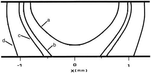
Table III. Summary of numerical model predictions of thermal damage (10% and 63% contours as indicated) for the Tm:YAG laser lesion at 5 and 50 s of heating. Calibration by collagen birefringence loss shows excellent agreement in this case for the thin tissue section. The damage/cell death bandwidth is indicated by 10–90% ΔR (mm).
Figure 9. Tm:YAG laser PC3 cell death field at t = 8 s. Inner contour (a) is 63% cell death by the (slower) Arrhenius calculation (and corresponds to the 72 °C contour at 5 s) and the outer contour (b) is 63% cell death (Ω = 1) by the two-state model prediction (and corresponds to the 61 °C contour at 5 s).
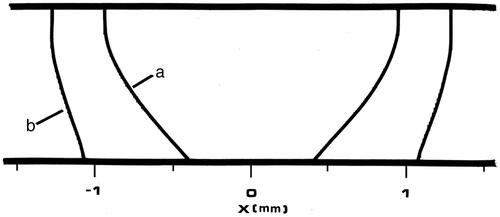
Figure 10. Plot of damage process predictions from 50 s of Tm:YAG laser heating analogous to . All four contours represent 63% damage (Ω = 1) for each damage process depicted, and the designations used in have been preserved. The innermost contour is collagen birefringence loss (a), the third contour is muscle damage and disruption (b), the second contour is PC3 cell death from the two-state model (c), and the outermost contour is loss of clonogenicity in S-phase CHO cells according to the Mackey model, (d). Note that the relative positions of contours (b) and (c) have reversed between the two figures.
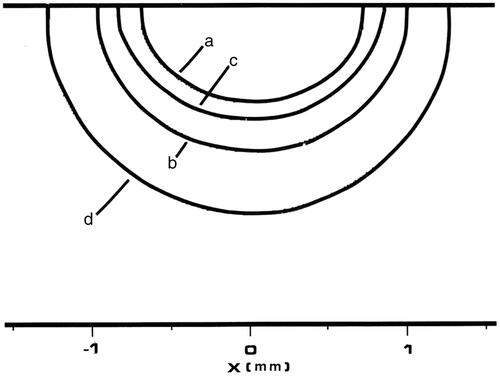
Figure 11. Comparison of the predicted rates of loss in CHO cell clonogenicity by the CEM and Arrhenius approximations. A) Rate of loss of clonogenicity, k, calculated from the Arrhenius relation (solid line), by using temperature-dependent RCEM(T) and D0(43) = 697.7 s (- - -), and by RCEM(43) = 0.477 and D0(43) = 697.7 s (- • - • -). B) The errors in the two CEM approximations (%) referred to the Arrhenius rate (%); temperature-dependent RCEM(T) (- - -) and RCEM = 0.477 (- • - • -).
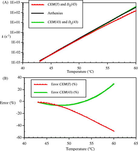
Figure 12. The dynamic response of A) the O’Neill et al. model at 90 °C and B) a comparison arbitrary reversible reaction model as in Equation (6) with constant coefficients of ka = 0.007, kb = 0.008 and kc = 0.01 (s−1).
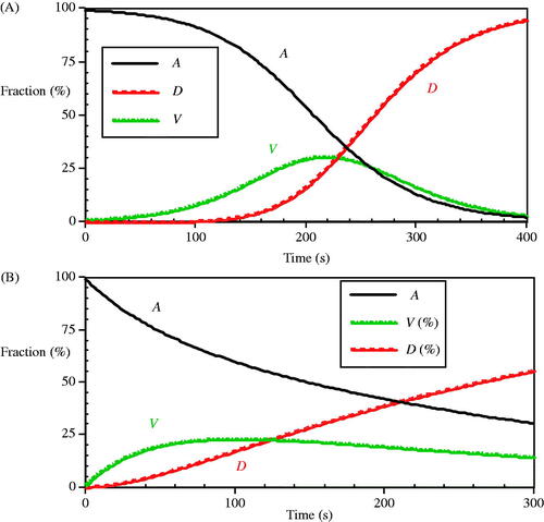
Figure 13. Plot of calcein signal loss in Dunning AT-1 tumour cell studies [Citation73]. Data points were extracted from mean values in of the publication. The Arrhenius fit was based on reported parameters (lines as indicated). In both cases the signal loss is over-predicted except for the longest heating times.
![Figure 13. Plot of calcein signal loss in Dunning AT-1 tumour cell studies [Citation73]. Data points were extracted from mean values in Figure 2 of the publication. The Arrhenius fit was based on reported parameters (lines as indicated). In both cases the signal loss is over-predicted except for the longest heating times.](/cms/asset/2b664939-e6f9-4345-9d08-b622d0b67343/ihyt_a_786140_f0013_b.jpg)
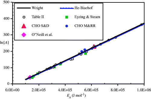
Figure 14. Plot of coefficients from (open circles) and Eyring and Stearns’ enzyme measurements (solid squares) compared to Equations (17a) (solid line) and (17 b) (dashed line, barely distinguishable). Also shown are the Sapareto and Dewey CHO cell (large solid triangle), Mackey and Roti Roti coefficients (solid circles), and Arrhenius coefficients for the O’Neill et al. data as calculated for this paper (large solid diamond at left end of plot).