Figures & data
Figure 1. A graphical illustration of the non-linear constitutive model [Citation27] used for the perfusion and optical absorption is shown. The scattering behaves similar to the absorption. Damage, perfusion, and absorption are plotted as a function of a time–temperature history representative of those observed in MRgLITT procedures. As shown, the native undamaged constitutive values transition into coagulated constitutive values between temperatures of approximately 51–61 °C. Similar to previous results [Citation49], the tissue is fully damaged at a threshold of 61 °C.
![Figure 1. A graphical illustration of the non-linear constitutive model [Citation27] used for the perfusion and optical absorption is shown. The scattering behaves similar to the absorption. Damage, perfusion, and absorption are plotted as a function of a time–temperature history representative of those observed in MRgLITT procedures. As shown, the native undamaged constitutive values transition into coagulated constitutive values between temperatures of approximately 51–61 °C. Similar to previous results [Citation49], the tissue is fully damaged at a threshold of 61 °C.](/cms/asset/2464cd00-8465-498b-b9b9-030d02286a71/ihyt_a_798036_f0001_b.jpg)
Table I. Literature-based constitutive values [Citation46,Citation50–52,Citation54,Citation55, Citation77–80] A table of the constitutive values used for perfusion, conduction, absorption, and scattering is shown. Uniform distributions are denoted U(a,b). Deterministic values are otherwise used. Values for density, specific heat, and Arrhenius parameters are as follows: ρ = 1045 (kg/m3), cblood = 3840 (J/kg/K), cp = 3600 (J/kg/K), A = 3.1E98 (1/s), EA = 6.28E5 (J/mol), R = 8.314 (J/mol/K).
Figure 2. These plots are spatial profiles that demonstrate the properties of a stochastic BHTE, with inputs listed in . A is a linear sensitivity study; each colour represents data from a univariate model, i.e. one parameter is varied while all others are constant. A has the following plots, listed from low to high variance at peak heating: perfusion (fuchsia), conductivity (green), optical scattering (blue), optical absorption (red), and optical anisotropy (violet). The parameters’ relative sensitivities can be seen in this figure. For example, perfusion is proportionally varied more than the optical absorption and scattering parameters, but the optical parameters still have a greater temperature variance. The BHTE is most sensitive to the anisotropy factor in this study. B and C are a sensitivity study comparing linear and non-linear perfusion parameters; For B and C, the solid lines represent the CDF = 2.3 and 97.7%; the enclosed region is the central 95% confidence interval. B has optical absorption (red and green with dashed lines) and scattering (fuchsia and blue with solid lines) while C has perfusion. The linear cases’ inputs vary the concerned parameter over a range that includes both the native and coagulated states of the non-linear case. The plots demonstrate coagulation affecting the temperature distributions. D simultaneously varies optical scattering, optical absorption, conductivity, and perfusion. The difference between the worst-case scenarios (black) and CDF = 1% and 99% (red) is shown.
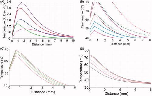
Figure 3. The trivariate joint uncertainty of the optical absorption, scattering, anisotropy are input for the gPC simulations. Model parameters are listed in . A is the MRTI of the phantom study at t = 90 s. The inner red contour is the 50 °C isotherm for the model’s mean and the outer red contour is for the CDF = 97.3%; CDF = 2.3% never reaches 50 °C. The dark blue contour is the MRTI’s 50 °C isotherm. Only one MRTI isotherm is displayed because the MRTI variance is very small; ± 2σ of MRTI noise is ∼2 °C. The black rectangles in A, B, and D occlude where the laser fibre was. The superimposed green line represents the location for linear profiles B and D. A green diamond indicates the location of the temporal profile in C. D compares the linear profile of the central 95% confidence intervals of the model and MRTI. In plot D, the model’s mean tracks very well with the MRTI, particularly near the laser fibre (±∼6 mm). D also dramatically shows the potential for non-Gaussian distributions to arise in the temperature model, further illustrated in B. B shows various CDF values tracked in the gPC computer package, DAKOTA. The top red is CDF = 99%, green is the median (50%), red dashed line is the mean, violet is 5%, black is 2.3%, bottom red is 1%. Note the extreme skewness of the model’s temperature output near the fibre, as evidenced by the mean and median being much nearer the higher percentage CDFs than the lower percentage CDFs. The power, displayed as green points, is provided units on the right vertical axis of C.
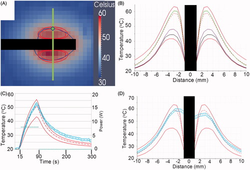
Figure 4. These temporal profiles, A through D, are temporal profiles from canines 1 through 4, respectively. The red and blue dashed and solid lines represent the same mean and CDF values listed in . The green points represent the power history. The spatial locations of the temporal profiles are shown in via the green diamonds. A and D show the best agreement of the four plots. B is more successful at the beginning of the imaging sequence but the model is much colder at later time points. C tends to be somewhat cooler, but significant overlap remains between the MRTI and model distributions.
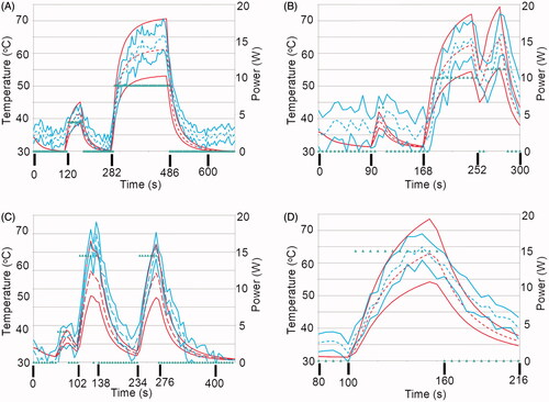
Figure 5. Plots A through D correspond to canines 1 through 4 at the same time points described in . A also contains a perfusion univariate model that uses optical scattering and absorption from white matter tissue (violet). The black rectangles obfuscate the portions of the linear profiles that are on the laser fibres because those regions provide invalid comparisons. A suggests that white matter optical scattering and absorption parameters produce profoundly colder temperatures. In plots A and B the trivariate model tends to overlap the MRTI well. Plots C and D show some agreement near the fibre (±∼3 mm), but diverge at further distances.
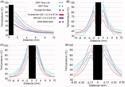
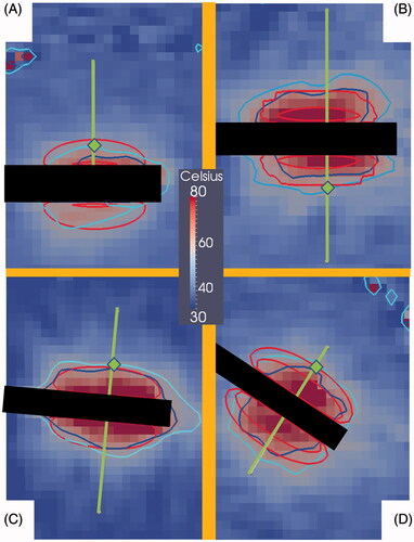
Figure 6. These images are MRTI from the four canine normal brain MRgLITT ablations. All images are from a slice that intersects the longitudinal axis of the laser applicator. Images A, B, C and D respectively correspond to canines 1, 2, 3 and 4 near maximum heating times t = 432 s, 222 s, 120 s, and 135 s. The superimposed green lines represent where the linear profiles for the four canines are plotted for Figures 4 and 5. Green diamonds indicate the location of temporal profiles in canine . The black rectangles in each image are where the laser fibres were. The concentric red contours correspond to the predicted 60 °C isotherm contours with probabilities CDF = 2.3% and 97.7%. The areas between the red contours represent the central 95% of the model’s temperature distribution. According to the model, the CDF = 2.3% contour has a high probability of occurring, i.e. 97.7%. The dark blue and light blue contours respectively are the 60 °C isotherms from the MRTI temperature ±2σ of MRTI noise.