Real-time infrared thermography detection of magnetic nanoparticle hyperthermia in a murine model under a non-uniform field configuration

Figures & data

Figure 1. (A) TEM picture of the manganese ferrite-based nanoparticle surface-coated with citrate (MNF-citrate). The inset shows the size distribution obtained from the analysis of the TEM data. (B) Magnetisation curve of the MNF-citrate nanoparticles. The upper inset shows the response of the magnetic fluid to a permanent magnet, while the lower inset is the X-ray diffraction pattern of the nanoparticles. (C) Mapping of the magnetic field in the non-uniform field experimental condition. (D) Magnetic field amplitude along the coil axis, i.e. for R = 0 mm and distinct z-values. (E) Temperature profile of the magnetic fluid sample for the in vitro study under distinct coil positions. (F) Specific loss power of the magnetic fluid sample for the in vitro study under distinct coil positions.

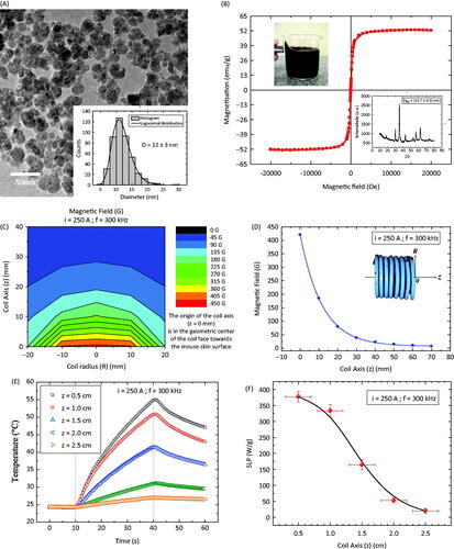
Figure 2. (A) Experimental set-up for the in vivo magnetic nanoparticle hyperthermia. (1) Computer, (2) Fibre-optic thermometer, (3) Alternating field generator, (4) Infrared thermal camera, (5) Coil, (6) Animal lift. (B) Schematic representation of both temperature measurements, namely from the thermal camera (surface) and fibre-optic (surface or intratumour).

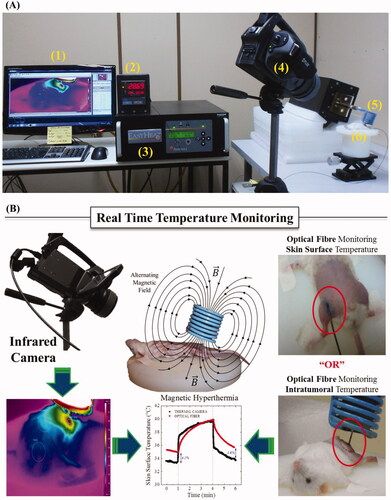
Figure 3. (A) Thermal camera image of a healthy animal without magnetic fluid before turning on the field. (B) Same animal after 3 min of hyperthermia, field on. (C) Thermal camera image of a healthy animal after a magnetic fluid injection before turning on the field. (D) Same animal after 3 min of hyperthermia, field on. (E) Temperature increase for the different cases investigated, i.e. eddy current (EC) for the healthy animals, magnetic nanoparticle hyperthermia for the healthy animals (MNP, healthy), eddy current in tumour animals (EC, S180) and magnetic nanoparticle hyperthermia in tumour animals (MNP, S180).

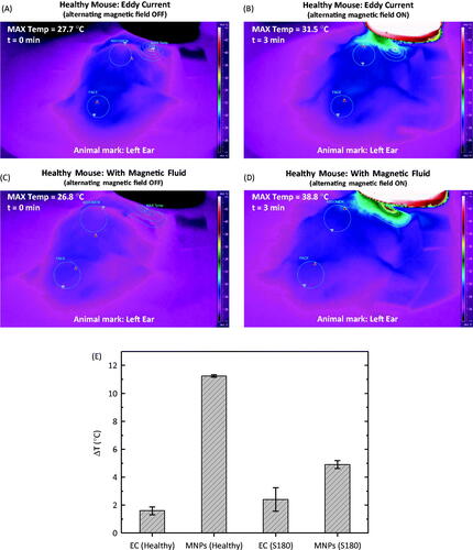
Table 1. Parameters obtained from the hyperthermia treatment procedure.

			Skin surface temperature									Comparison of hottest region on tumour with
Animal identification			Hottest region on the tumour (°C)			Face (°C)			Abdomen (°C)			Face (°C)	Abdomen (°C)
Animal	Condition	Type	Tmin	Tmax	ΔT	Tmin	Tmax	ΔT	Tmin	Tmax	ΔT	ΔTmax	ΔTmax
1	Healthy	EC	29.20	30.60	1.40	28.90	28.90	0.00	27.70	29.70	2.00	1.70	0.90
		MNPs	28.31	39.62	11.31	27.50	27.60	0.10	27.20	28.70	1.50	12.02	10.92
2	Healthy	EC	29.58	31.37	1.79	28.50	29.00	0.50	29.00	30.70	0.80	2.37	0.67
		MNPs	28.57	39.75	11.18	28.10	28.20	0.10	27.90	29.00	1.10	11.55	10.75
3	S180	EC	31.10	32.90	1.80	28.40	28.90	0.50	29.90	31.10	1.20	4.00	1.80
		MNPs	29.70	34.80	5.10	29.00	29.00	0.00	29.70	31.40	1.70	5.80	3.40
4	S180	EC	30.50	32.50	3.00	29.20	29.80	0.60	30.30	31.80	1.50	2.70	0.70
		MNPs	28.70	33.40	4.70	28.50	28.90	0.40	28.20	30.30	2.10	4.50	3.10

Time for each experiment was 3 min.

Table 2. Parameters obtained from the hyperthermia treatment procedure of 30 minutes.

Animal identification				Skin surface temperature									Comparision of hottest region with		Intratumoral
Ear	Physical	Type of	Time of	Hottest region on the tumour			Face			Abdomen			Face	Abdomen	Temperature
marked	condition	MH	MH Δt	Tmin (°C)	Tmax (°C)	ΔT (°C)	Tmin (°C)	Tmax (°C)	ΔT (°C)	Tmin (°C)	Tmax (°C)	ΔT (°C)	ΔTmax (°C)	ΔTmax (°C)	Tmin (°C)	Tmax (°C)	ΔT (°C)
2 LEFT	S180	MNPs	30 min	28.00	39.30	11.30	29.50	31.00	1.50	29.10	31.00	1.90	8.30	8.30	30.40	38.99	8.59

Figure 4. (A) Thermal camera image of an animal with a S180 murine tumour after a magnetic fluid injection before turning on the field. (B) Same animal after 5 min of hyperthermia, field on. (C) Same animal after 12 min of hyperthermia, field on. (D) Same animal after 30 min of hyperthermia, field on. (E) Same animal 1 min after turning off the field. (F) Time-dependent temperature profile at different animal positions. The thermal camera extracted information of the maximum temperature close to the injection region, the face, and the abdomen of the animal. Conversely, the fibre-optic thermometer measured the intratumoral temperature during the hyperthermia procedure.

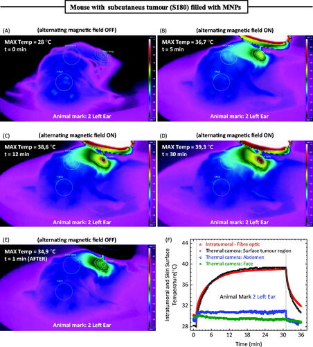
Figure 5. (A) Ex vivo animal image showing the S180 tumour. (B) Ex vivo animal image after removing the tumour. (C) Ex vivo images of the tumour. (D) Tumour dimensions, volume and mass.

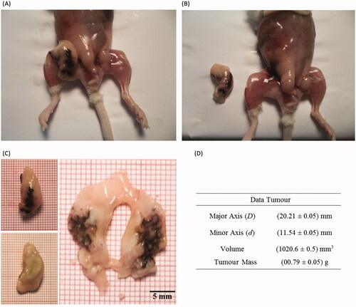
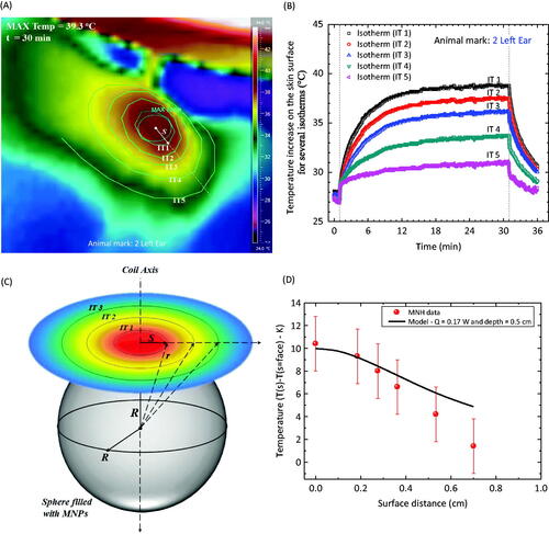
Figure 6. (A) Thermal camera image of an animal with a S180 murine tumour after a magnetic fluid injection after 30 min of hyperthermia. The image is a close look in the region near the magnetic fluid injection. Several isotherms are identified. (B) Time dependence temperature profile at different animal positions, i.e. for the distinct isotherms. (C) Schematic representation of the nanoparticle organisation inside the tumour. (D) Symbols represent the temperature increase, after thermal equilibrium (30 min), at distinct isotherm positions. The solid line is the theoretical calculation using the simplified model discussed in the text.