Validation of MR thermometry: Method for temperature probe sensor registration accuracy in head and neck phantoms

Figures & data

Figure 1. Head and neck hyperthermia phantom set-up. (a) Top view of phantom. (b) Side view of phantom showing catheter path. (c) Fibre-optic temperature probe strand containing four equi-spaced temperature sensors distributed along its length. (d) Illustration of phantom set-up: the temperature probe strand from (c) is inserted into the catheter track which has a non-linear trajectory through the oil and phantom interior. Right magnification box: due to the bending catheter trajectory it is common for the temperature probe tip to become stuck before reaching the actual catheter tip. This will lead to temperature probe/MRT data misregistration (see text for further discussion).

Figure 2. 3D spline catheter mapping. (a) Coronal fast-SPGR image showing the catheter in the phantom. For images such as this, the tip localisation was within <1 mm accuracy (in-plane uncertainty in the catheter tip was within 1 pixel on a 512×512 matrix with 33 cm FoV). Also shown here are the approximate axial slice locations for the SPGR images used in the MRT calculations. Axial slices are labelled 1–4. (b) Spline fits for catheter/temperature probe localisation. Data points are extracted from images such as (a) to reconstruct the catheters in MR image coordinate space.

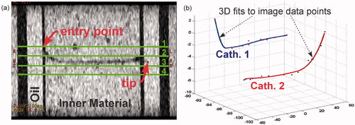
Figure 3. Heating array and axial MRT images. (a) MR-compatible heating array. The phantom sits inside a hollow water bolus cylinder. Patch hyperthermia antennas radiate phase-coherent RF at 434 MHz for heating. (b) Fat-referenced axial PRFS MRT map for slice 2 from Figure 2(a) showing general temperature probe sensor locations. Sensors 1–3 are part of one temperature probe for which the tip is located to the left of ‘3’. Sensors 4–6 are part of another temperature probe for which the tip is located to the right of ‘4’. Despite having four total sensor points per fibre-optic strand, during the experiments only three were usable, as one sensor was located in the fat/oil ring and therefore displayed no temperature-dependent phase change. The data for the sensor point located in the fat/oil is not shown.

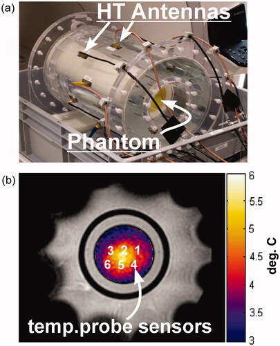
Figure 4. Sensor localisation and alpha calibration. (a) Shows the method used to determine temperature probe strand displacement inside each catheter. Each point on the plot represents the Pearson product-moment correlation (R²) of a linear regression line from a plot such as (b), where the PRFS phase change for all the sensors in a given catheter are plotted as a function of ground-truth temperature at a specific position along the spline curve. As you can see in (a), when the R² ∼ 1 (as indicated by the grey line) the temperature probes are localised correctly inside the catheters. Here the temperature probe in catheter 1 is shifted ∼13 mm, while the temperature probe in catheter 2 is shifted ∼20 mm as indicated by the arrows. (b) PRFS phase is shown as a function of ground-truth temperature for all sensors non-localised: i.e. assuming 0 mm difference in registration between the catheter and the temperature probe tips. Here R² < 0.900. (c) PRFS phase is shown as a function of ground-truth temperature for all sensors localised: i.e. after the sensors in temperature probe 1 have been shifted 13 mm and the sensors in temperature probe 2 have been shifted 20 mm from the catheter tip as indicated in (a). Here the R² > 0.998. The slope of this curve is the PRFS thermal coefficient (α-parameter).

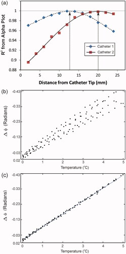
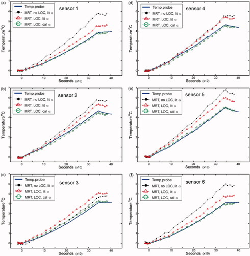
Figure 5. Heating experiments performed with ‘gelatin’ phantom. (a–f) The temperature data has been plotted for sensors 1–6 respectively, as depicted in Figure 3(b). On each plot, the ground-truth temperature data is represented by the solid blue curve. MRT data is also shown on each plot. Solid black circles represent MRT data processed for non-localised (no LOC) sensors assuming a literature PRFS-thermal coefficient (α-parameter) value of 0.01 ppm/°C (lit α). Hollow red triangle points represent MRT data processed for localised (LOC) sensors assuming a lit α. Hollow green circle points represent MRT data processed for localised (LOC) sensors with a calibrated α value of 0.0123 ppm/°C (cal α) from the slope of Figure 4(c). Similar results were obtained with the ‘superstuff’ phantom.