
Figures & data
Figure 1. The H&N HT prototype MRT pilot set-up. (A) Schematic. (B) Simulation model. (C) Coil placement. (D) Coronal registration scan, indicating the external and local fat references and the top and bottom thermal probe sensors.
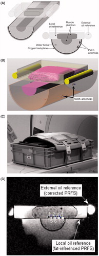
Table 1. Dielectric and thermal properties (434 MHz, 20–30 °C) as used in EM and thermal simulations. εr is relative permittivity, σeff is effective conductivity, ρ is mass density, cp is the specific heat capacity and k is the thermal conductivity.
Figure 2. Heat distribution plotted as an overlay on the MR image, measured at various time points (indicated in ) in the 2D plane using three PRFS methods, compared with a thermal simulation result (bottom). The (red) line in the fat-referenced PRFS and simulation plots indicates the 50% isotherm of fat-referenced PRFS at t = 1066 and binds the area of interest for the statistical analysis shown in .
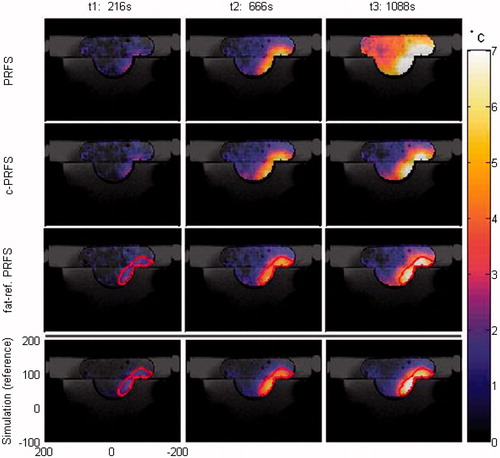
Figure 3. Temperature–time characteristic of MRT results, compared with a reference taken at probe 8 (see ). Dashed lines indicate the time points where the data of were obtained.
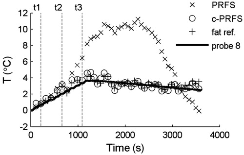
Table 2. Accuracy (root mean square error εrms), precision (standard deviation σ), range (maximum error εmax) and correlation (squared correlation coefficient r2) of the various MRT measurements, using probe measurements (above the line) or temperature simulations (below the line) as a reference. All values are given in °C, except r2 which is unitless.